
Dieser Abschnitt enthält Einführungsvideos für die Hardware, die Thales-Software und die Zahner-Analysis-Software.
IM7

Meet Our New IM7 with Zahner Lab ()
Produktvideo der Potentiostaten-Familie IM7 (IM7c, IM7, IM7x) mit der Software Zahner Lab: die Geräte, ihre Fertigung in Deutschland, Messungen und Prüfstandsintegration.Textfassung: Meet Our New IM7 with Zahner Lab
Produktvideo der Potentiostaten-Familie IM7 (IM7c, IM7, IM7x) mit der Software Zahner Lab: die Geräte, ihre Fertigung in Deutschland, Messungen und Prüfstandsintegration.
Automatische Abschrift
Produktvideo mit Musik und ohne Sprache. Die eingeblendeten Texte sind englisch. Texte und Szenen der Reihe nach:
- „Meet Our New IM7 with Zahner Lab“ (unsere neue IM7 mit Zahner Lab)
- „Exceptional Hardware for Electrochemistry with a New Soul“ (außergewöhnliche Hardware für die Elektrochemie mit neuer Seele): Die drei Geräte erscheinen nacheinander.
- IM7c, „Compact and Precise“ (kompakt und präzise): ±5 V und ±14 V, ±2 A in 12 Strombereichen, EIS-Bereich von 10 µHz bis 5 MHz.
- IM7, „Powerful and Modular“ (leistungsstark und modular): ±5 V und ±15 V, ±3 A in 12 Strombereichen, EIS-Bereich von 10 µHz bis 8 MHz, bis zu 5 synchrone Kanäle.
- IM7x, „The Ultimate Platform“ (die ultimative Plattform): ±5 V und ±15 V, ±4 A in 12 Strombereichen, EIS-Bereich von 10 µHz bis 12 MHz, bis zu 33 synchrone Kanäle.
- IM7c / IM7 / IM7x: 32-Bit-DC- und 24-Bit-AC-Auflösung, schnelle Datenerfassung, Gigabit-Ethernet-Anschluss.
- „Made in Germany“, 50 Jahre Erfahrung in der Impedanzspektroskopie, hohe Fertigungstiefe der Elektronik am deutschen Standort: Leiterplatten werden bestückt, geprüft und in ein Gerät eingesetzt.
- Eine IM7 und ein PP242 messen neben Referenz-Multimetern.
- „Software Zahner Lab“: Ein Impedanzspektrum (Bode- und Nyquist-Diagramm) baut sich während der Messung auf.
- Eigene Experimente erstellen, volle Freiheit beim Messablauf: Ein Experiment wird aus Blöcken zusammengesetzt.
- EIS bis 40 A / 400 kHz (IM7 / PP242), bis 680 A / 100 kHz (IM7x / EL1002), bis 4000 A (IM7x / FRA-X / Fremdgeräte).
- Parallele Messung mit PAD42, bis zu 33 synchrone EIS-Messungen, 24-Bit-Auflösung auf allen Kanälen.
- Alternative Signalverarbeitung: nichtlineare Frequenzganganalyse, Zeitbereichsanalyse, Operando-EIS.
- Prüfstandsintegration mit zahner_link, Bibliotheken in C++ / Python für alle gängigen Betriebssysteme, WebSocket-Protokoll: Fernsteuerung mit JSON-Objekten; Prüfstände in einer Fertigungshalle.
- „Join Us on the Journey of Investigating Electron Transfer on All Scales“ (begleiten Sie uns bei der Erforschung des Elektronentransfers in allen Größenordnungen)
- „Precision in Electrochemistry“ (Präzision in der Elektrochemie)
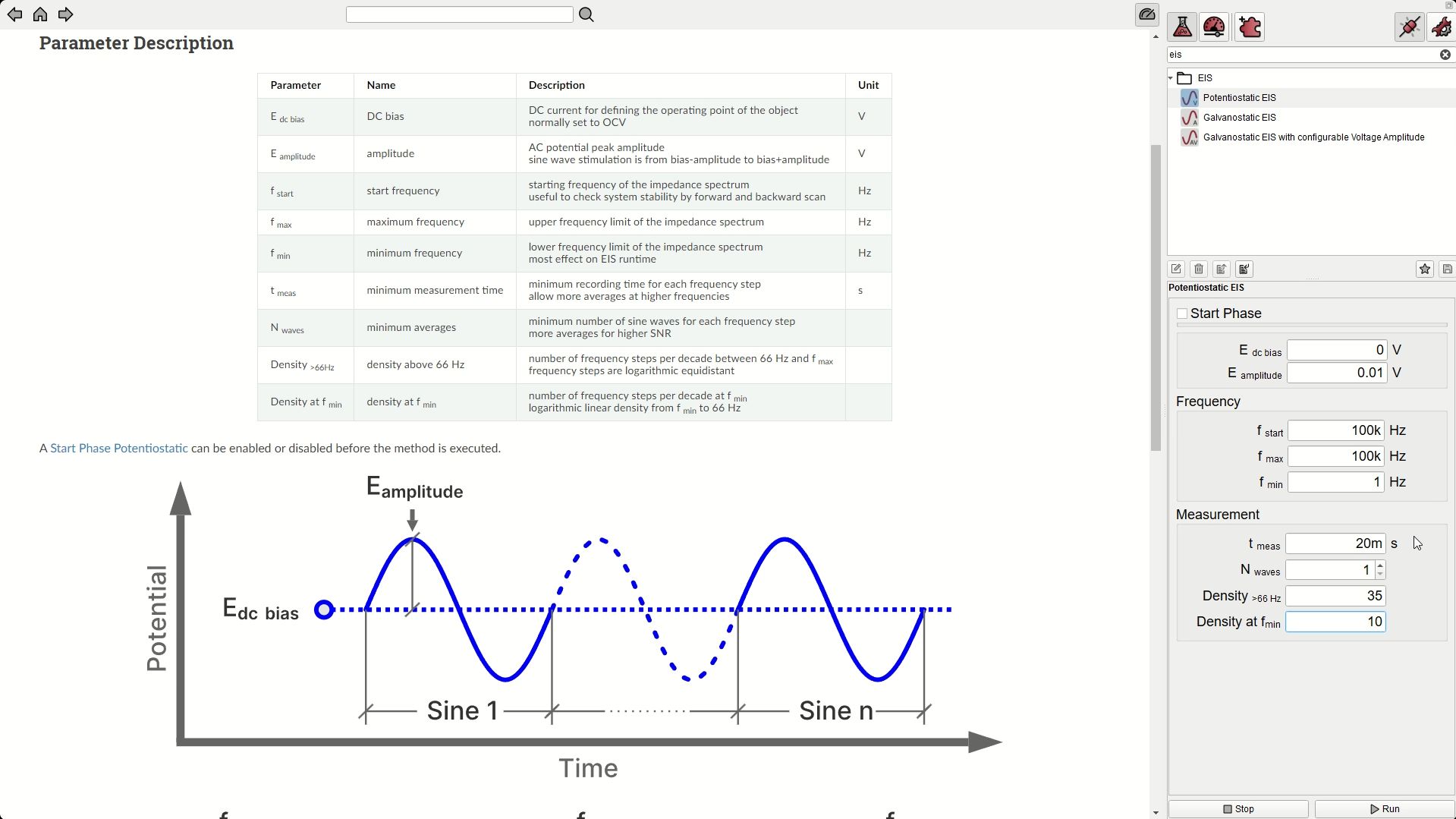
Electrochemical Impedance Spectroscopy (, ohne Ton)
Bildschirmaufnahme: eine potentiostatische EIS-Messung in Zahner Lab, von den Parametern bis zum Bode- und Nyquist-Diagramm.Textfassung: Electrochemical Impedance Spectroscopy
Bildschirmaufnahme: eine potentiostatische EIS-Messung in Zahner Lab, von den Parametern bis zum Bode- und Nyquist-Diagramm.
Bildschirmaufnahme in Zahner Lab: Die Parameter einer potentiostatischen EIS-Messung (Start-, obere und untere Frequenz, Messzeit, Anzahl der Wellen, Punktdichte) werden neben ihrer Beschreibung eingestellt. Dann läuft die Messung, und Bode- und Nyquist-Diagramm bauen sich Punkt für Punkt auf, während Impedanz, Phase und Frequenz angezeigt werden.
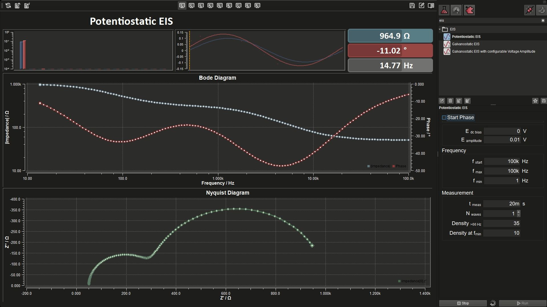
Zahner Lab: Dark Mode (, ohne Ton)
Bildschirmaufnahme: dieselbe EIS-Messung im dunklen Modus von Zahner Lab.Textfassung: Zahner Lab: Dark Mode
Bildschirmaufnahme: dieselbe EIS-Messung im dunklen Modus von Zahner Lab.
Bildschirmaufnahme: dieselbe potentiostatische EIS-Messung im dunklen Modus von Zahner Lab. Die Parameter werden eingestellt, dann bauen sich Bode- und Nyquist-Diagramm während der Messung auf.
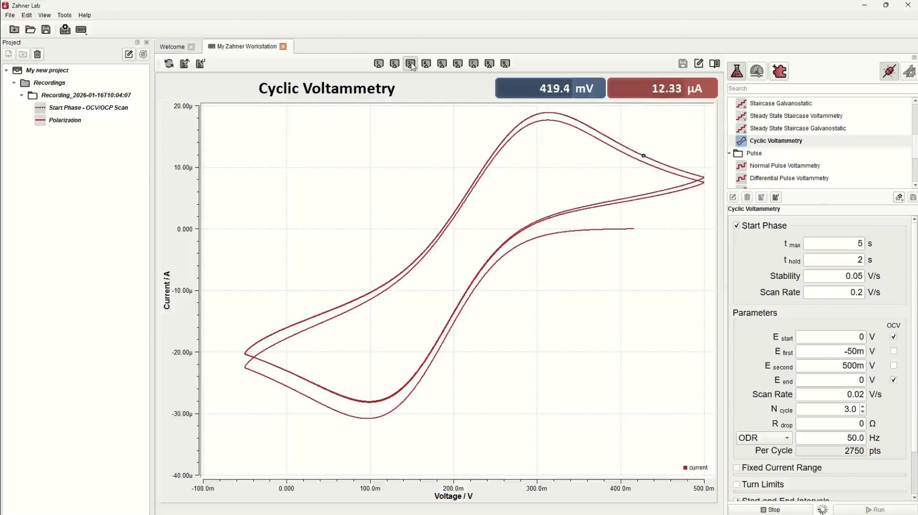
Cyclic Voltammetry (, ohne Ton)
Bildschirmaufnahme: eine zyklische Voltammetrie in Zahner Lab, von den Parametern bis zum Voltammogramm.Textfassung: Cyclic Voltammetry
Bildschirmaufnahme: eine zyklische Voltammetrie in Zahner Lab, von den Parametern bis zum Voltammogramm.
Bildschirmaufnahme in Zahner Lab: Die Parameter einer zyklischen Voltammetrie (Start-, Umkehr- und Endpotenzial, Scanrate, Anzahl der Zyklen) werden neben einem Diagramm des Potenzialverlaufs eingestellt. Dann läuft die Messung: Das Voltammogramm sowie Potenzial und Strom über der Zeit werden live gezeichnet.
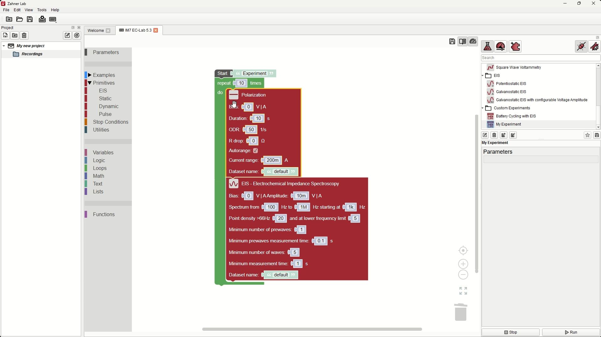
Custom Experiment Builder: Easy Example (, ohne Ton)
Bildschirmaufnahme: In Zahner Lab wird ein einfaches eigenes Experiment aus Blöcken gebaut.Textfassung: Custom Experiment Builder: Easy Example
Bildschirmaufnahme: In Zahner Lab wird ein einfaches eigenes Experiment aus Blöcken gebaut.
Bildschirmaufnahme in Zahner Lab: Aus einem leeren Arbeitsbereich wird ein neues eigenes Experiment angelegt. Blöcke für eine Polarisation und eine EIS-Messung werden hineingezogen und eingestellt, dann wird eine Schleife um beide gelegt, die sie wiederholt.
Custom Experiment Builder: Complex Example (, ohne Ton)
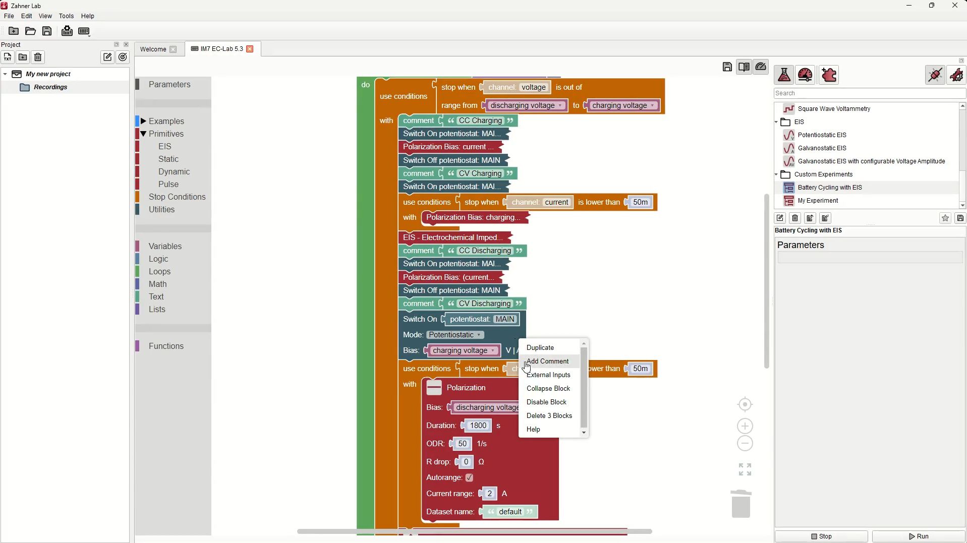
Bildschirmaufnahme: das eigene Experiment „Battery Cycling with EIS“ in Zahner Lab.Textfassung: Custom Experiment Builder: Complex Example
Bildschirmaufnahme: das eigene Experiment „Battery Cycling with EIS“ in Zahner Lab.
Bildschirmaufnahme in Zahner Lab: Das fertige eigene Experiment „Battery Cycling with EIS“ wird geöffnet und durchgescrollt. Eine Schleife lädt und entlädt eine Batterie mit Konstantstrom- und Konstantspannungsphasen, beendet jede Phase über Spannungs- und Stromgrenzen und führt nach jedem Schritt eine EIS-Messung aus.
Custom Experiment Builder: CV with Different Scan Rates (, ohne Ton)
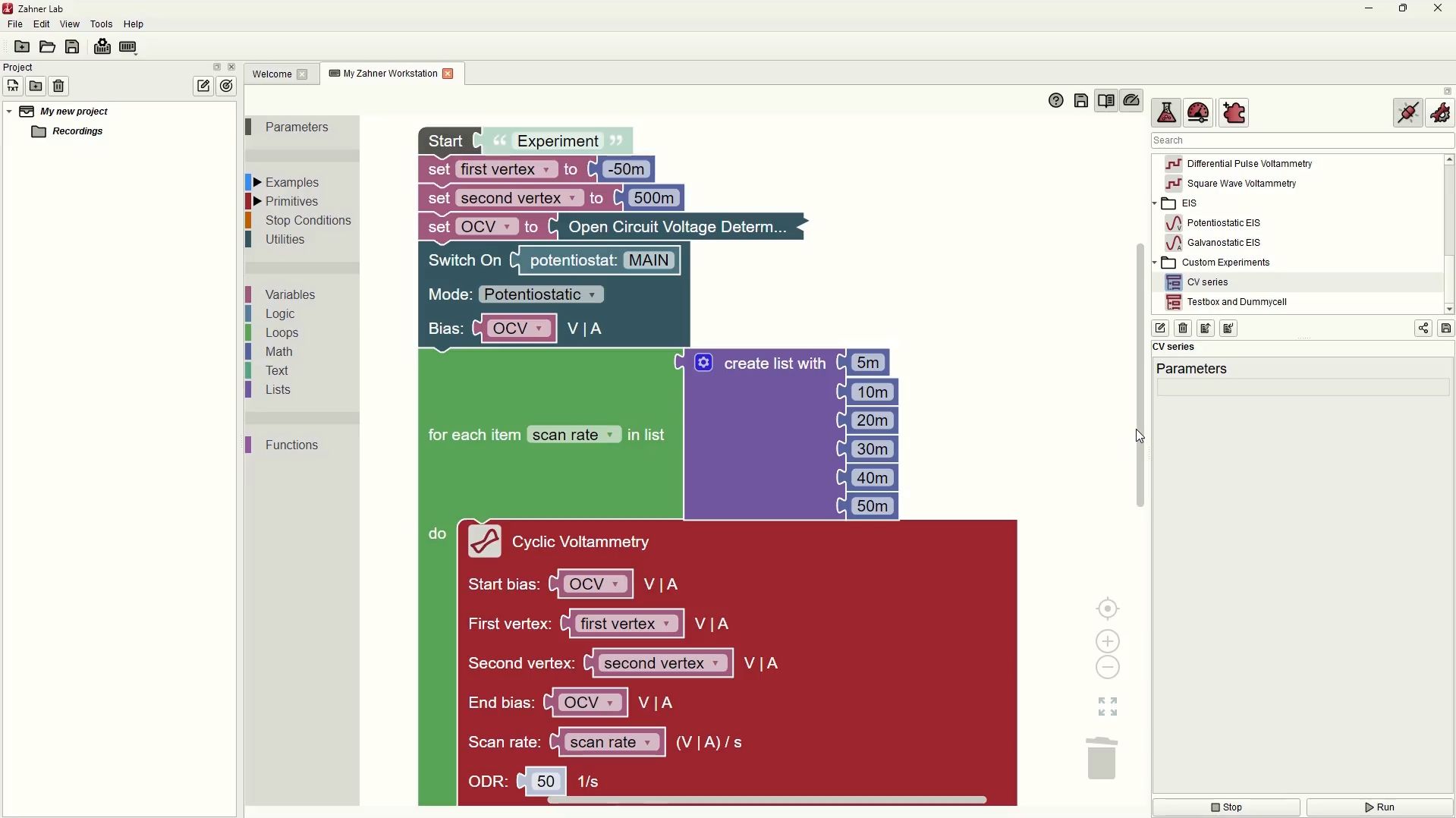
Bildschirmaufnahme: Ein eigenes Experiment in Zahner Lab misst zyklische Voltammogramme bei fünf Scanraten.Textfassung: Custom Experiment Builder: CV with Different Scan Rates
Bildschirmaufnahme: Ein eigenes Experiment in Zahner Lab misst zyklische Voltammogramme bei fünf Scanraten.
Bildschirmaufnahme in Zahner Lab: Ein eigenes Experiment führt für jede Scanrate einer Liste (5, 10, 20, 30 und 40 mV/s) eine zyklische Voltammetrie aus. Die Voltammogramme aller Scanraten werden nacheinander in ein Diagramm gezeichnet.
Technische Videos

Unboxing eines ZENNIUM-Potentiostaten ()
UnboxingTextfassung: Unboxing eines ZENNIUM-Potentiostaten
Unboxing
Automatische Abschrift
Hello everyone and welcome to this video of Zahner. My name is Waqas Saddique. I'm an application specialist and marketing manager here in Zahner. Today in this video I'm going to unbox a ZENNIUM PRO parcel for you. I'm going to show you that when you order a ZENNIUM PRO from us, what accessories does it comes with. At this point I would like to say that irrespective of which potentiostat you order, either it is ZENNIUM X, ZENNIUM PRO or ZENNIUM XC, the accessories are going to be the same. This means that if you order a ZENNIUM XC or ZENNIUM X, the accessories will stay the same and this video is relevant also for you.
So with this let's get started. You can see here that I have already opened the ZENNIUM PRO parcel and the first thing we have is this Zahner ZENNIUM file and when you open this file, we have the Zahner Analysis license sheet. This analysis license sheet contains the license keys and you can use this license key to activate your Zahner Analysis software. The next we have is Thales user manual and this user manual will help you in getting started with your device. It tells you that how to install the Thales software and how to install the Zahner Analysis software and then how you can connect this ZENNIUM potentiostat properly with your laptop, with the main power supply and how to get started with the experimentation. At the right here we have this USB. This USB contains the latest version of the Thales software and the Zahner Analysis software so you can install them. In addition to that, it also has the calibration data for your device.
Here in Zahner, each and every potentiostat is individually calibrated. That means each and every potentiostat has its own calibration data and the calibration data for your device is within this USB. You can see that at this USB, we have a small sticker and this sticker contains the serial number of your device and the same serial number is also on your potentiostat. So you can check which USB belong to which potentiostat and then you know that this calibration data belongs to this device. So let's say in future you install a newer version of the Thales software, then after the installation of this software, you have to install the calibration data again. So it is very important that in future you keep this USB safe so that you can install the calibration data. Okay, so that was the first accessory. The next thing we have is a small box and this box, first of all, contains this USB cable. You will use this USB cable to connect your ZENNIUM potentiostat with your laptop or your computer.
Next we have this power cable which you will use to connect your ZENNIUM potentiostat with the main power supply. Then we have this test box. If you want to check the performance of your ZENNIUM potentiostat, you can connect this test box to your ZENNIUM potentiostat and do a routine diagnostic check and this will tell you the performance of your ZENNIUM potentiostat. At the end, we have two sets of cell cables. So one of these long cell cables which are one meter long cell cable. So these are one meter long cell cables as you can see and these cell cables we have four different colors. So we have four cell cables which are this black one is for the working electrode, blue one for the working electrode sense, green one for the reference electrode and this red one is for counter electrode.
And then in addition to that, we have the shorter cell cables. So make sure that you have these two sets of cell cables with you in the accessories. So these were the accessories and now I will take out the ZENNIUM PRO potentiostat out of the box. As you can see here that I have already taken out the potentiostat out of the box. This is some dry material for security. And then on the right side, we have an important warning from the electrostatic discharge. With this we came to the end of our video. I unpack the ZENNIUM PRO parts for you. I showed you all the accessories that it comes with.
In my next video, I will talk about the front panel of the ZENNIUM PRO potentiostat or a ZENNIUM potentiostat. And then in particular, we will discuss this warning about electrostatic discharge and what the user should take care of. With this, I thank you for your time and see you in the next video.
Frontplatte des ZENNIUM-Potentiostaten ()
Textfassung: Frontplatte des ZENNIUM-Potentiostaten
Automatische Abschrift
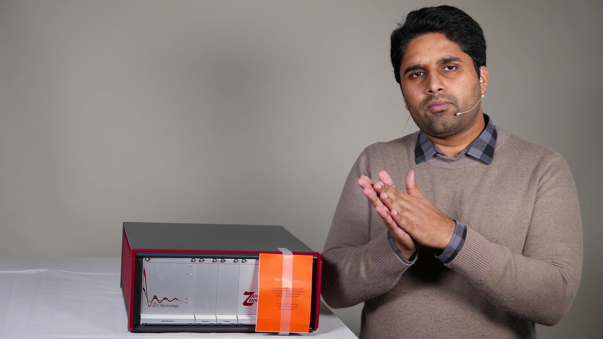
Hello everyone and welcome to this video of Zahner. My name is Waqas Saddique. I'm an application specialist and marketing manager here in Zahner. Today in this video I'm going to introduce you to the front panel of this ZENNIUM potentiostat. When you order a potentiostat from us, you take it out of the box. This is what you get. The first thing we will see on the front panel is this warning sign. This warning sign is about electrostatic discharge. What is electrostatic discharge? If you are making some movement, there is a friction between your clothes and your body, so you gather some charge. If you're working on a mat, there is a friction between your shoe, sole, and the mat, so you gather some charge. And whenever you touch a metallic part, you have, you get this shock and then what you do is that you transfer your charge to the metallic body. And now let's say that your body is charged, and you try to connect the cell cable here with your BNC connectors.
And what you will do is that when you come here, you will have electrostatic discharge and you will expose your potentiostat to very high voltage. And this might damage your potentiostat. So that's why whenever you try to connect your cell here, first of all, touch the body of the ZENNIUM potentiostat so that you discharge yourself, and then connect your cell cables. With this, you, you emit this possibility that you will have electrostatic discharge near the BNC connectors. If you have an ESD mat, you can have an ESD mat on your table, put your ZENNIUM PRO or ZENNIUM potentiostat on that ESD mat, and then touch the mat before you proceed with working with the potentiostat.
So this was this warning sign was about that always discharge your body of any charge, and then proceed to working with the potentiostat. Now let's talk about the right side of the potentiostat. Here we have the four BNC connectors. And these BNC connectors are to connect your electrochemical cell with the potentiostat. So these four connectors are for the working electrode, for working electrode sense, for reference electrode and for the counter electrode. And then on the very right, we have I-probe and E-probe. So let's say that you have an electrochemical cell or a system which has very high impedance, and you want to do impedance spectroscopy, so EIS on the system. What you need is you need a probe from us, which is used for doing impedance at this very high impedance system. And this is called high impedance probe, and you will connect this probe at I-probe and E-probe and other side of the probe will be connected to your cell. So this is one extreme, high impedance. If you go to the other extreme, you have low impedance systems. And if you want to do a measurement at low impedance, you need a low impedance probe that will again will be connected here at I-probe and E-probe and other side of the probe will be connected to your system under investigation. So these are this probe. If you want to do some special experiments, you need some help. And this help is comes from these probes which are connected here.
Then in the middle, we have extension slots. If you want to extend the power of your ZENNIUM potentiostat, you can use a power potentiostat. And this power potentiostat can be connected to the ZENNIUM PRO or ZENNIUM X, Y and extension cards. And these extension card will be installed here. Then let's say that you order your ZENNIUM potentiostat already with the power booster, then the cards will come already installed. But let's say that you have a ZENNIUM or ZENNIUM PRO. And later on, you decided that you want to have a power booster, you order a power booster from us, you order the extension card, and then you can simply remove these screws.
And you will take out this metallic part and you will just plug, put in your card and they are plug and play. That means you just plug them in and they are good to go. Okay, and then on the very left side, we have the CPU of our potentiostats or the brain of our potentiostat. And here if you have bought your potentiostat before 2020, then you will see that there were two switches. These switches must always be at go if you want to use the ZENNIUM potentiostats. And there was this possibility that somebody accidentally turn off the switch and bring it at stop and then they try to use the potentiostat and it will not work. So these switches have to be at go. And then to mitigate this possibility that somebody will just turn off the switch, remove the switch and the function of the switch is now carried on by the software. When I will be talking about the Thales software, I will also introduce you to this new function which is done by the software. Okay, so that was a quick introduction to the front panel of the ZENNIUM potentiostat. We talked about the BNC connectors, we talked about the I and E probe and extension cards. If you order a ZENNIUM XC, there are no possibility to extend. So this part is not available in the ZENNIUM XC. And then we talked about the brain, the CPU of our potentiostat. In my next video, I will talk about the back panel of the potentiostat. I will talk about how you can properly set up the grounding of the electrochemical cell or the potentiostat and how to avoid the ground loop. With this, I thank you for your time and see you in the next video.
Rückseite des ZENNIUM-Potentiostaten ()
Textfassung: Rückseite des ZENNIUM-Potentiostaten
Automatische Abschrift
Hello everyone and welcome to this video of Zahner. My name is Waqas Saddique, I'm an application specialist and marketing manager here in Zahner. Today in this video I'm going to introduce you to the back panel of the Zahner ZENNIUM potentiostat. In particular I will talk about how to set up the grounding properly and how to avoid the ground loop. We will start from the left side and what you see here is a small sticker. And this sticker tells you that which kind of potentiostat do you have.
Here we have a Zahner ZENNIUM PRO and below that there is a serial number written for this device. So whenever you contact us regarding your potentiostat, it's always better for us to know which serial number you have so that we can identify your potentiostat. And if you do not know where the serial number is, it is written on the sticker at the back panel. Now we come on the right side. On the right side we have the connection for the mains where you will connect your wire.
Then we have the power switch and then on top of that we have a fuse. If you look carefully here there is a number written. This number should correspond to your voltage of your mains. For us this is 230 V. Let's say for you it is not 230 but 115. Then you have to remove this fuse and make sure that it is at 115 V. For this take something like a screwdriver, push this button up and as you push this up this pop out. And now just above this number we have these two fuse. One of them has this smaller circumference, the other one has this bigger part.
So I will just push this out and now you see that at the bottom there is 230 written and 115 written. So if it is 115 for you, you will put that in in such a way so by turning it around that now here 115 is written. But for me 230 was correct so I will just turn it once more and then push it in and now again it is 230 here. And once 230 is there or the correct voltage for you is there you will just push it in.
Keeping in mind that this push button is at the bottom and then just plug it in back. So you have to give here a bit force. Make sure that your potentiostat is off, the wires are removed. Now here at the top we have the USB connection so this white one here. With this you will connect the ZENNIUM potentiostat with your laptop. At the bottom we have the grounding and the floating switch. So if your electrochemical workstation is at the grounding conditions then you have to click here at the floating.
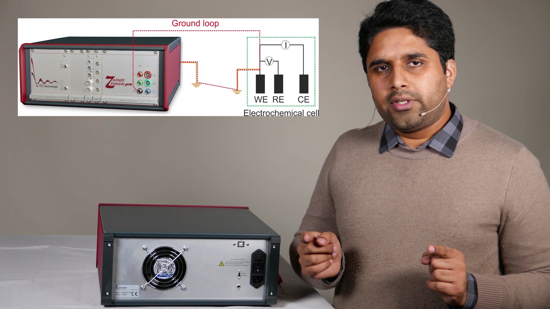
And if your electrochemical workstation is at the floating conditions which is mostly the case then you will turn this back to the grounding. The potentiostat is grounded via the power cable so this is grounded. Now you have to make sure that one of your potentiostat or your electrochemical cell only one is grounded. If both of them are grounded then the current going from the potentiostat will not go through the cell but will go through this ground loop and you will have problems. So make sure that only one of them is grounded and this way you will meet the problem of ground loop.
Okay the last thing we have here this fear 4 millimeter terminal. This 4 millimeter terminal is used if you want to ground something else besides your potentiostat. For example you are working with a Faraday cage and this Faraday cage has to be grounded. So you have your Faraday cage somewhere and you connect a wire through this Faraday cage and you connect this via here. What this does is that this will extend the grounding of the potentiostat to your Faraday cage. If you are using ESD mat you can also ground that here.
Do not ground this part to somewhere in your lab. If you take a wire connected somewhere in the lab at the ground potential and put this wire here then you will have a ground loop within the potentiostat and that will also create problems. So this small inlet is for extending the ground of this machine of this potentiostat to the Faraday cage. So this was a quick overview of the back panel of the ZENNIUM potentiostat. We talked about the grounding conditions and how you can avoid the ground loop.
In my next video I will install the Thales software and the calibration data so that we can start with the software. So with this I thank you for your time and see you in the next video.
Thales-Software
Installation der Thales-Software ()
Textfassung: Installation der Thales-Software
Automatische Abschrift
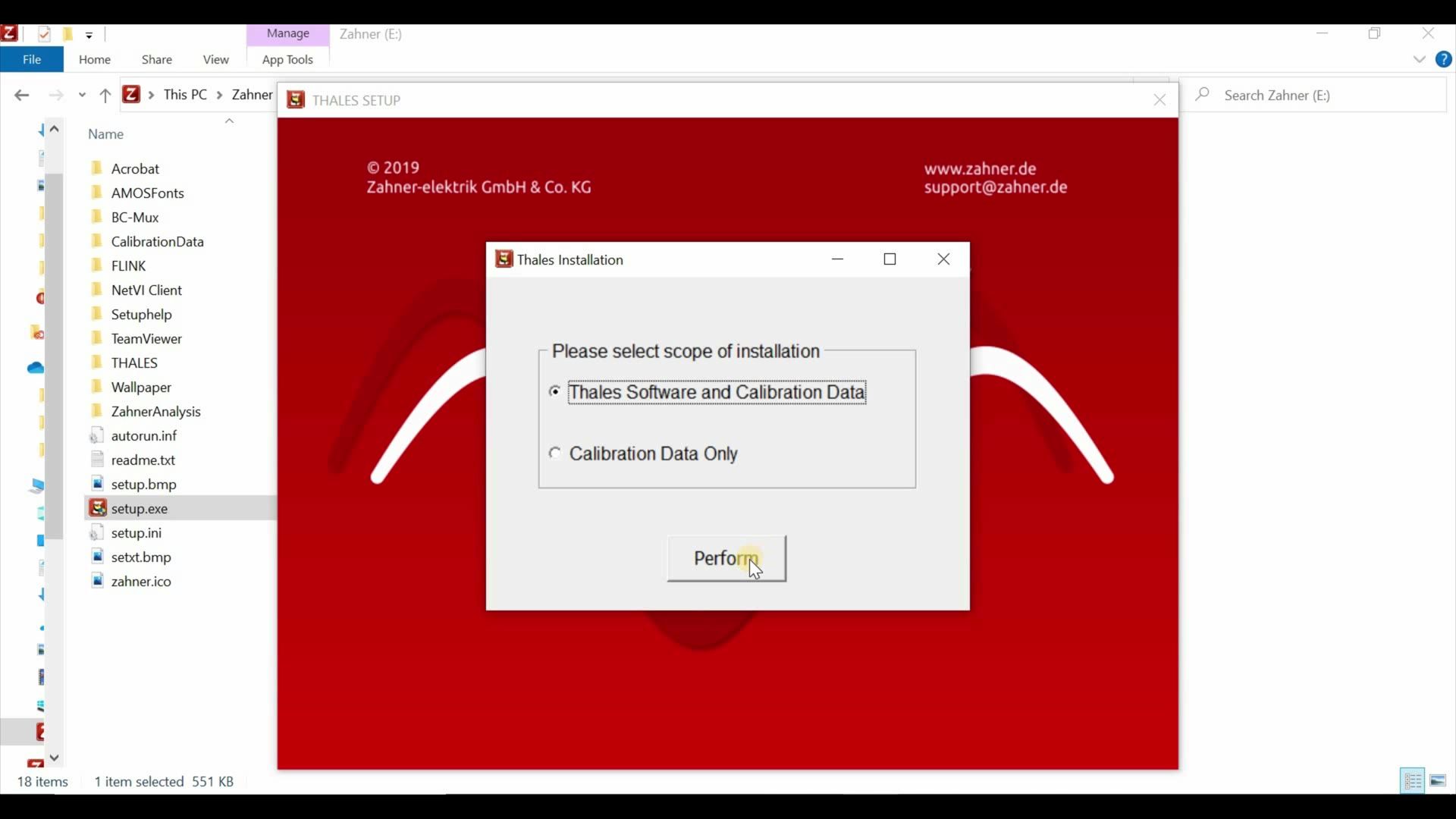
Hello everyone and welcome to this video of Zahner. My name is Waqas Saddique. I'm an application specialist and marketing manager here in Zahner. Today in this video I'm going to show you that how you can install the Thales software, how to install the calibration data for your device and how to install the Zahner Analysis software. So with this let's get started. You got a USB with your Zahner, ZENNIUM, potentiostat. Go ahead and plug that USB into your computer. As you plug your USB you will see that you have the Zahner drive there. Just open that drive and this is what you will see. Now to start the installation process I will click on setup.exe. So double click it opens a new window and in this window it asked me do I want to install the Thales software and the calibration data or do I want to do the calibration data only.
For today we will install the Thales software and then the calibration data. But let's say in future you have a newer version from us and after the installation of the newer version of the Thales software you want to install the calibration data only then you will click here. But for today we will install the Thales software and then you will click perform and then it asks you do you want to have some other software for example the BC-Mux or Adobe Acrobat reader and it will also create a desktop icon. So I will just click here installation and now what you see here we have Thales XT 5.6.2. This is currently the latest version. In future if you have later version then you install that software you can ask us and then we will send you a link for the software. Install the software same way it is done here and then you can induce the USB to install your calibration data. Now click next to install the drivers it's very fastly done click finish and then again next and then it's also finished. Now there is an option to choose the language English is always default but you can also go to Deutsch and then this is German.
But for today we will stick with English you click OK and then it installed the BC-Mux because initially we also said we want to install the BC-Mux software. I will click next and it checked that I already had the BC-Mux and it said do you want to install it so I will say yes and then I will click next and install my BC-Mux software. I do not want to launch the BC-Mux software currently so I will just click on finish. Now it automatically start the next software which was Adobe Acrobat Reader. Now it checked that I already had an advanced version of the Adobe Acrobat Reader so it will says that you already have a better version so it will stop.
Finished and now it start with the Zahner Analysis so the third software of course it already have this current version which is the latest version. If the later version comes up you can always ask us and we will send you a link with the latest version. So you click next you agree of course here all the files should be ticked because then the Zahner Analysis can accommodate all these different file types and then you click next and install. And now it will start installing the Zahner Analysis software it always very fast it might need you like two to three minutes to go through the whole process if you just click next and finish. So I'm done with installation and now it asks me do I want to have a classic mode or the Thales XT mode. You can choose whatever you want but it's not as if that later on you cannot change between these two it is very easy to go from XT mode to the classic mode. I will talk about this in a future video but for today we can just click on classic mode and just click continue. Again it asks you for the language for the Thales software and then you click install. Now you can see that this was installing the calibration data and then you click finish and you are good to go the installation has been completed. So now we are done with the installation of the Thales software Zahner Analysis software and the calibration data.
In my next video I will show you that how you can properly connect all the wires with the potentiostat, how to connect an electrochemical cell and how to do a measurement. With this I thank you for your time and see you in the next video.
Einführung in die Thales-Software ()
Textfassung: Einführung in die Thales-Software
Automatische Abschrift
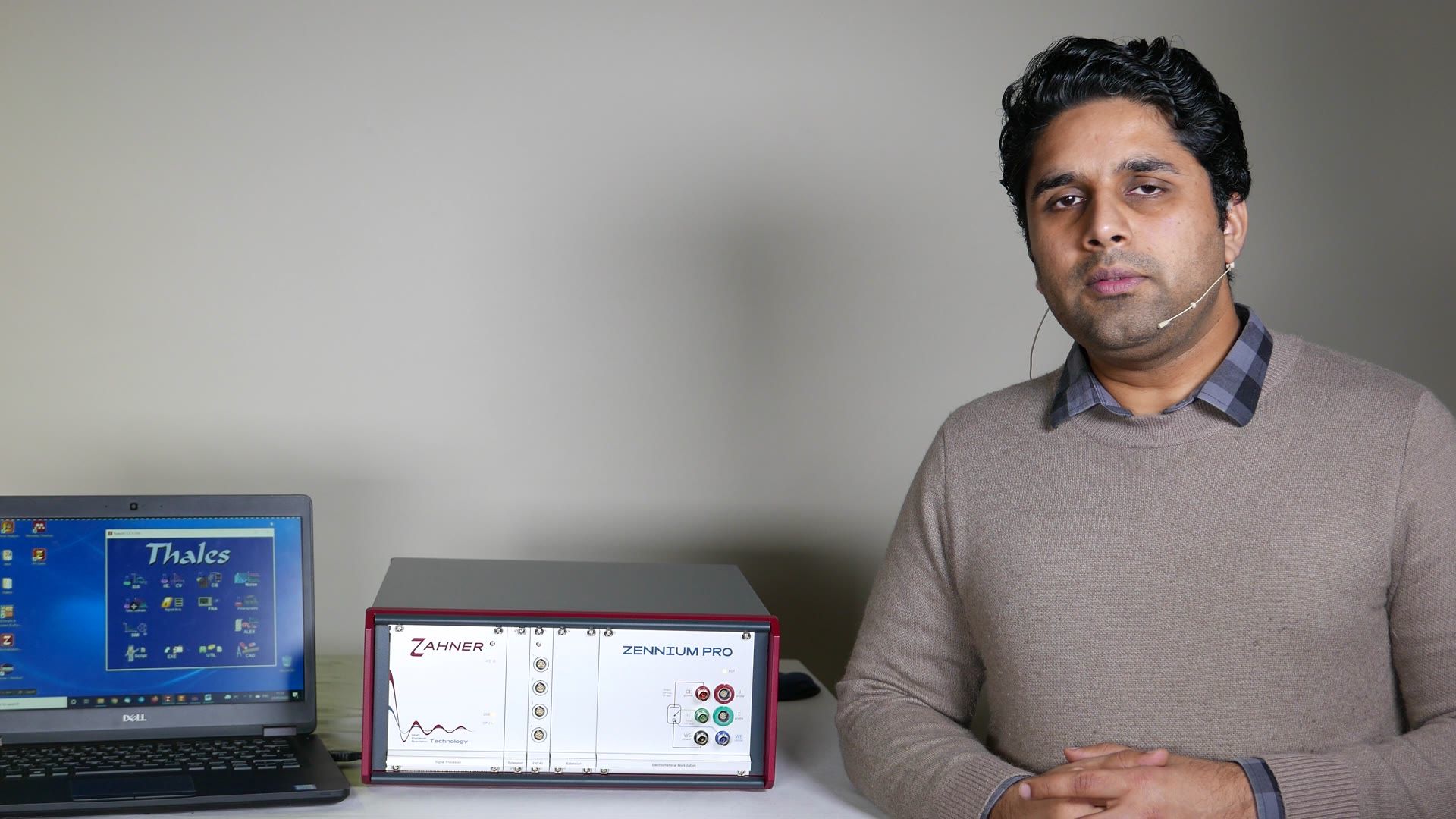
Hello everyone and welcome to this video of Zahner. This is Waqas Saddique. In this video, I'm going to introduce you to the Thales software. In my last video, I showed you how you can install the Thales software. If you haven't checked out that video, you can find the link in the description below. Before we start up the Thales software, you need to connect your ZENNIUM series, potentiostat or if you're working with an older version of the ZENNIUM potentiostat, for example an IM6 potentiostat, you need that connected with your computer.
So connect the power cable to the potentiostat and a USB cable which is connecting the potentiostat to your computer where you install the Thales software and then power up the potentiostat and now you can start your Thales software. So the Thales software will not turn on if you are not connecting it with the potentiostat. So for using the Thales software, the potentiostat have to be connected and have to be turned on. Now with this, let's go to computer and see how you can start up the Thales software.
To start up the Thales software, double click on Thales USB icon.
As the Thales software starts up, the first notification you will see is the warm-up of the potentiostat. When you are working in your lab, we advise you to wait 30 minutes of the warm-up so that you can use the potentiostat in the optimum condition. For today we will just start with the Thales software and what you see in front of you is the Thales classic mode. It could be that you are looking at the gray window and that gray window is our Thales XT mode and that you can look at if you go to the Z and switch to XT mode. Here is the Thales XT mode in a future video. I will talk about each and every function of the Thales XT mode but today we want to go back to Thales classic mode. So now we are back in the Thales classic mode and you can see here that we have different kind of icons and each icon represent their own kind of measurement. So you have impedance spectroscopy and here you can do electrochemical impedance spectroscopy and then you have I/E, CV icon where you can do current voltage measurements or cyclic voltage measurement.
And then on the third we have CE icon. These are capacitance potential measurements. So if you are doing single frequency impedance measurement you can calculate capacitance from it so you can do something like Mott-Schottky curve. You can do noise measurements and then you can also do is in the second line you have the time domain measurement. So you can apply some voltage with time and you can look how the current is behaving or you can apply current and look at the voltage. So any measurement with respect to time can be done here like square wave voltammetry and then you have signal acquisition. So we in Zahner we offer different kind of extension possibilities. We offer different kind of cards and these cards provide you analog and digital input and output channels and these channels are then controlled in signal acquisition.
Other than that we have many different kind of icons and in future I will talk about them. Today let's focus on impedance spectroscopy. If you click on impedance spectroscopy icon you get to the second window and in this window you see the parameter regarding the impedance spectroscopy. So you have your frequency range, you can apply a frequency, you can choose your steps per decade, how many measurements you want to do in one decade. A very nice feature of Thales is that if you go to some variable and right click with your mouse it opens up the manual of the Thales software at the correct position where you can read about that variable. Now let's try once again. I go to the steps per decade, I right click and now you can see again that I'm on the same page where the steps per decade are explained. Okay so this is the second part of the Thales software where the parameters are explained. So on the first level we have the main measurement techniques.
If I go to CV and click on CV I go to the second level where the parameter regarding cyclic voltammetry are explained. We have the first level of the measurement and second level of the parameters and then each of them have a third level of control potentiostat. So when you click on the control potentiostat to come to the third level of the Thales software and you can test your sample as the name suggests test sampling and potentiostat control. So what you can do you have a sample and you don't know how high the currents will flow at some specific voltage.
You can provide a voltage and you can look how high the currents are. So for example here I can provide, so I have high impedance sample connected to my potentiostat I provide one volt and I can look at the current which are about 10 nanoamperes and the asterisk here tells you the control parameter. So right now I'm applying one volt so the asterisk is on the voltage. I can turn off my potentiostat and I can go to galvanostat and once I do that the voltage which you see on the left side will be changed to current and as you see I choose to galvanostat and the voltage changed to current and now I can apply current. Here since I have a high impedance sample I can write 15 nanoampere so n here then stands for nano you can also write some value in 0.0 and so on but if you put n that stands for nano if you put u that is micro m for milli and so on and so forth.
So today I will give 15n click okay and turn on my potentiostat and as I do that the asterisk will now come on DC current and as you can see I can give 15 nanoampere current and I'm looking at the voltage which I'm measuring. Okay beside this we have many other things which we will talk about in future videos we have calibration and check cell connection schemes which will also be discussed in the future video. So now what I want to show you are some additional methods which are available in the Thales mode so you go to the optional methods in the drop down menu and here you see some additional measurements so if you are working remotely let's say you are controlling your system via python and c++ you can use our remote control application if you are working with coating or laminates you can do overcoating a laminate test if you are working with batteries you can do cycling of the batteries with battery cycling and then the very first option is photoelectrochemical test and this option is used and these are not one test but many tests and these are used by the customers who have our CIMPS system or the CIMPS extension systems.
So here you have then the additional measurements which are possible. Okay so with this we came to the end of our video in the next video I will talk about the front panel of the benches that we have few LEDs on the front panel I will show you what these LEDs are trying to tell us and how you can properly start up the Thales software. So with this thank you for your time and see you in the next video.
Starten der Thales-Software ()
Textfassung: Starten der Thales-Software
Automatische Abschrift
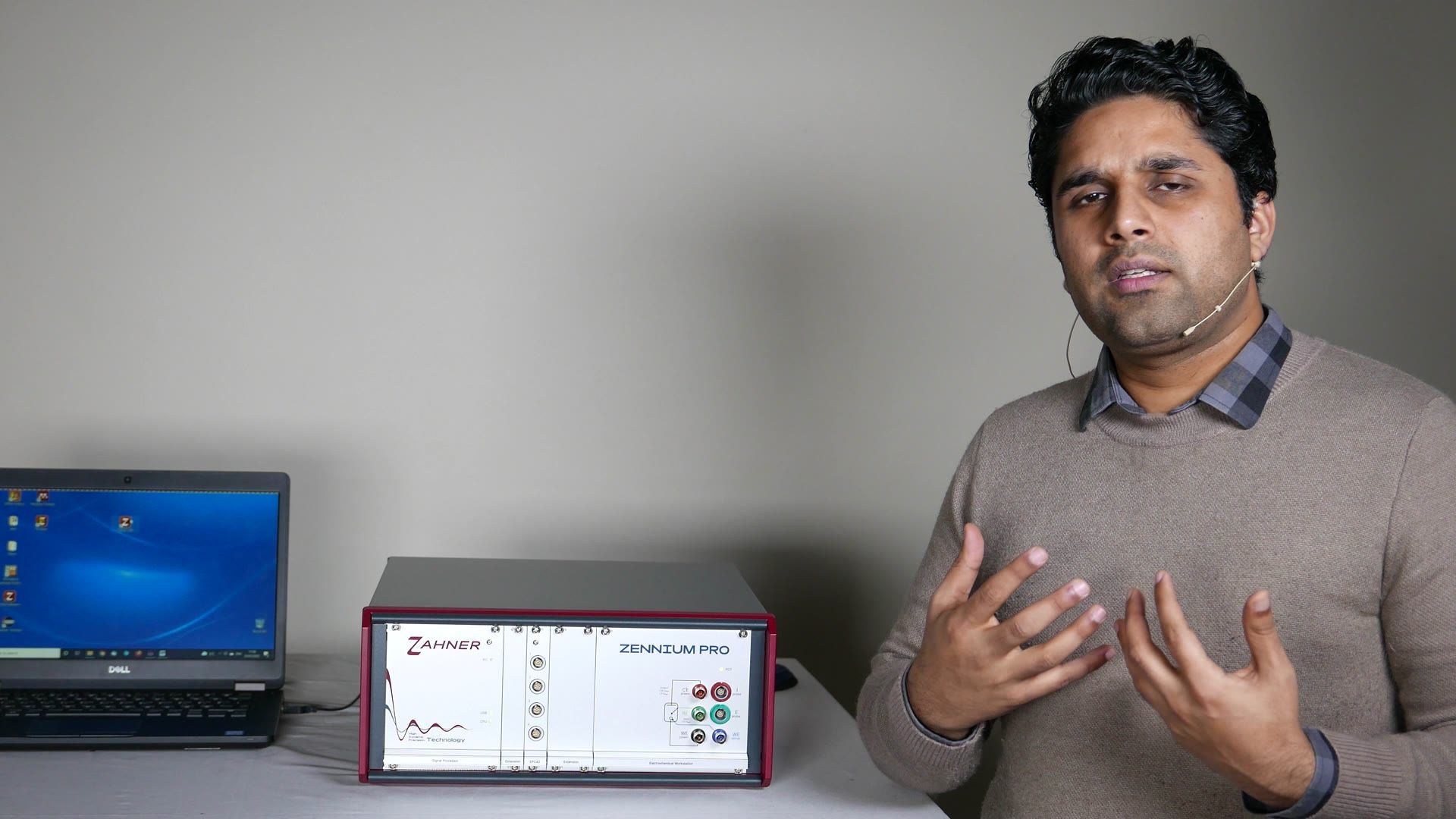
Hello everyone, and welcome to this video of Zahner, this is Waqas Saddique. In this video I am going to talk about the front panel of the ZENNIUM potentiostat, in particular I will be talking about the LEDs on the front panel and what they are trying to tell us. So when you have started up your ZENNIUM potentiostat, you see three LEDs, one here is the POT, POT LED and two LEDs are here, one is the USB LED and the second one is CPU LED. So once you have started up your potentiostat, we have not started up your software at this point, all three LEDs are green. Most important one here is at this point is the USB LED. So the green signifies that there is a successful connection between potentiostat and the computer.
And this tells me that now I can start my software. So when I will start the Thales software, this green LED will convert to orange. So I just started my Thales software and we see that the green LED changes to orange and this means that a successful connection has been built up. So when we are doing some measurement, there is some online signal processing going on. And for this, it is very important that the signal processor within the potentiostat and software are in sync with each other. Now let's say that I was working on my software, I was doing measurement and due to some reason, I turned off my software. So for example, I turned off it myself or there was some screensaver on my computer and the windows just shut down.
Now the software and the machine, the potentiostat are not in sync anymore. And now if I want to, so let me just close my software once again. And now I want to start my software again. But now if I see at my USB LED, it is orange and it is not green. So this tells me that they are not in sync right now. So if I want to make them in sync so that my software start up properly, then I can start up my Thales software. So very normally as you did before and then click on the Z icon and this will open a drop down menu. And the very last option is NMI reset handling. And here you go to the full reset and you do full reset. Now during the full reset, the potentiostat will be momentarily off and then it will turn on momentarily showing the both LEDs as green and your software will start once again automatically.
And this time the software ensures that it is in sync with the potentiostat. So by resetting, you are actually restarting your potentiostat and your software. And now you can very well start your measurement again and both of them are increasing and you will not have any problem with your software. Now these are the new potentiostat. If you are using an old potentiostat from Zahner, then you do not have this system in the software. In this case, there are two switches here on the front panel. And for resetting, you want to push up your lower switch to the reset position and then let it go. For some time it will again then restart and then the both LEDs will be green and once they are green, you can start your software.
Now for the second part of the video, I want to come back to our Thales software and we will go directly to the control potentiostat window. Now at this point, the potentiostat is off and the POT LED is green. But what would happen if I apply here, let's say 0.1 volt and turn on the potentiostat. As you can see that as soon as I applied some voltage or some current into my software, this POT LED has turned to orange. This orange signifies that now the potentiostat is giving power to your sample or the current is flowing through your sample. So it is not advisable to remove the cable connected to the potentiostat. So if you want to connect your sample or remove your sample, look at the POT LED. If it is green, go ahead do it. If it is not green and if it is orange, make sure you turn off your potentiostat and then when it is gray, then disconnect the cables or connect the cables. With this, we came to the end of our video for today. In my next video, we will talk about the control potentiostat window in detail. I will show you the different features of the control potentiostat window. So with this, thank you for your time and see you in the next video.
Einführung in das Control-Potentiostat-Fenster ()
Textfassung: Einführung in das Control-Potentiostat-Fenster
Automatische Abschrift
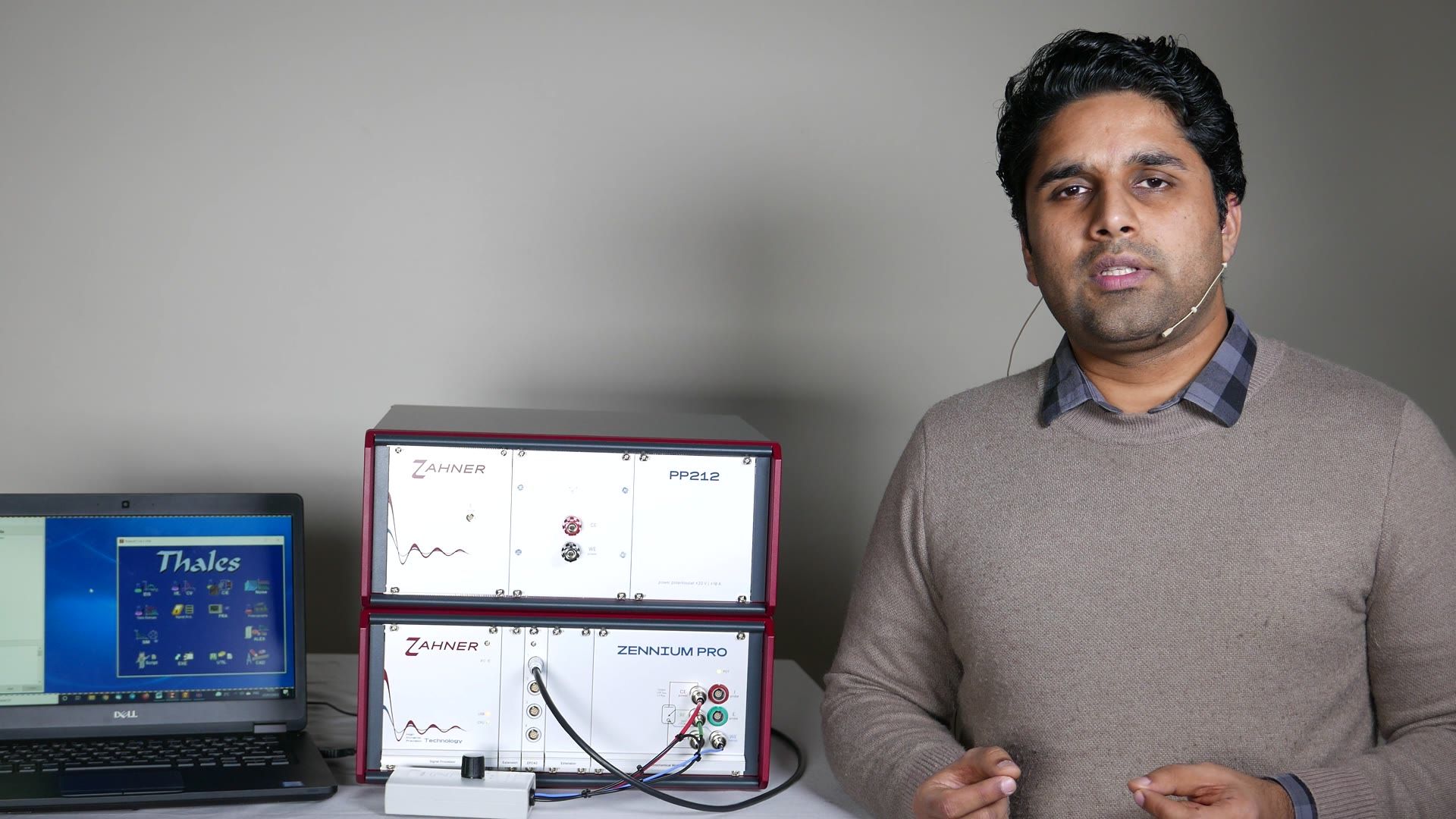
Hello everyone and welcome to this video of Zahner. This is Waqas Saddique. In this video, I want to talk to you about the control potentiostat window in the Thales software. But before we start with the software, let's have a quick look at the hardware which I have with me today. I have a ZENNIUM PRO potentiostat and have extended this ZENNIUM PRO potentiostat with the PP212 external potentiostat. Now I have already connected the potentiostat, the external potentiostat PP212 with mains via a power cable. And I also have the EPC cable which is connecting on one side the EPC42 card which is installed in or which is equipped with the ZENNIUM PRO.
And the other side of cable is connecting the back side of the power potentiostat. So with this, let's jump over to the software. Now here we have the Thales software. We want to talk about the control potentiostat window. So let's go to control potentiostat window. In my last video, I quickly showed you the control potentiostat window that we can apply here some voltage or some current to check the response of our test sample. So the bottom part is relevant if we are working with the impedance spectroscopy, but that is a topic for another video.
Now from here we have the device which is telling us the mains. So this is the main potentiostat that is ZENNIUM PRO potentiostat. Now if you remember from the start of video, I have connected the power potentiostat to the slot 1 of the EPC card. So I can go to device and I can go to 1 and I click OK. And now from here on main it's saying PP212. So it has detected PP212. And now if I give here some voltage, then that voltage will be delivered by the PP212 and not by the ZENNIUM PRO.
If you notice there is no change in the control potentiostat window. Only here you can see either you are controlling the main potentiostat or if you are controlling the power potentiostat or an electronic load. So if I go click on this device and I put 0 back and enter OK, then I go back to the main potentiostat and now these values which are being shown are for the main potentiostat. So now if I apply some voltage and turn it on, that power will be delivered by the ZENNIUM PRO and not PP212.
OK, the next part is the calibration part. So if I click on the calibration, I come to a sub window. If you are using an older version of the ZENNIUM potentiostats, then you will not have this window and as soon as you will click on calibration, it will just start the calibration or that will be the DC calibration. But for the newer versions, you have the possibility to calibrate for the DC measurements or calibrate for the AC measurements. We also have here high impedance measurement if you have HiZ-Probe and so on.
Here you have to keep in mind that if you want to calibrate your potentiostat, so all potentiostat which are delivered by us are individually calibrated. And when you install your Thales software, you also install the calibration data which was specific to your potentiostat. But for some reason, if you want to calibrate your potentiostat once again, make sure that you turn on your potentiostat, leave it for 30 minutes so that it's properly warmed up and then calibrate. Now if you want to save your calibration data, just click on save calibration. This will add the new calibration file in the folder where the previous calibration files are present.
Now if for some reason you want to go back to the original calibration files, you can go here and recall the previous calibrations. Next we have the check cell connections. If we click on check cell connection, here right now in the setting we have the main potentiostat and it is showing you that if you have some sample how you can connect the cable to this potentiostat. Now Zahner offers different kind of probes which you can connect with your ZENNIUM potentiostat. For example, you can have a HiZ-Probe and with this HiZ-Probe you can do measurement on high impedance sample.
Very nice feature in this window is that it also modify here this schematic and it shows you that how different cables must be connected. Our main potentiostat had two control voltage ranges, 5V range or 15V range. And if you need higher voltages you can just click here and now you will be in 15V range. Similarly here we have the compliance voltage so you can either work in 14V compliance volt or 28V compliance volt. And last but not least we have here reference electrode. So if you are using any reference electrode after the measurements you have to then modify your voltage axis.
Here you can do that automatically so you click on with reference electrode. You can see here again the schematic has been updated. Now with reference electrode if you try to go back it will ask you which reference electrode you are using. So you can choose one of this reference electrode from the list and let's say that reference electrode which you are using the voltage is not provided here. So you can click on user defined reference, click here on this tick mark and it will ask you what is the offset of your voltage and that you can provide here.
With this we cover most of the things which you can do with the test sampling window. And I thank you for your time and see you in the next video.
Einführung in Polarisationsmessung (POL) ()
Textfassung: Einführung in Polarisationsmessung (POL)
Automatische Abschrift
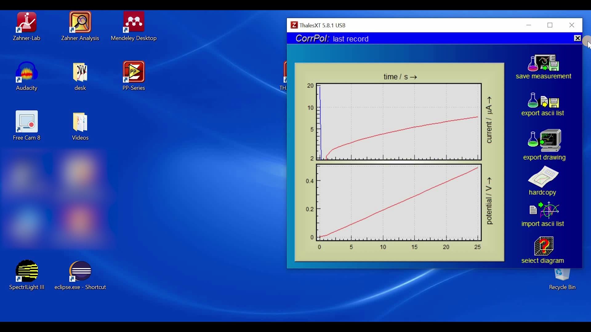
Hello everyone, and welcome to this video. This is Waqas Saddique. Starting today we are going to look at different techniques which we can carry out with Thales software. So I have already connected a ZENNIUM PRO potentiostat with my computer. I have turned it on and started my Thales software. As a dummy sample, I have connected the test box with the ZENNIUM PRO potentiostat and I have chosen the linear setting on my test box. Today we will be starting with the most simple kind of measurements that are the polarization measurements. So to start the polarization measurement hover your mouse on I/E, CV icon and then four sub icon will appear. And today we want to work with POL polarization so click on that. And with this you will come to the polarization window. As you can see we have here three phases phase one polarization phase two OCP scan and phase three is linear scan.
So we will unselect phase two and phase three and look at the phase one that is the polarization. In this phase one polarization I can apply a voltage. So here a voltage of 100 millivolt is given. I can maybe give 200 millivolt. The time of the measurement is one minute. You can change it by clicking on this time and this will open the time window. So I can put here maybe 30. So I can do this measurement in 30 seconds. So this is hours minute and seconds. And this delta T1 is the time difference after which a measurement will be recorded.
So I have only selected the phase one and here we have the current ranges. The ZENNIUM PRO has a current range of minus three to plus three ampere. For today we will select only the highest current range. Now I will start the measurement by clicking on start recording. Now the ZENNIUM potentiostat will apply 0.2 volt or 200 millivolt and it will measure current versus time. So the time was 30 seconds and you can see how the current is changing with time when we ever applied 0.2 volt. Now to save time I will just keep this measurement to the end. So the measurement just finished. You can click here to save your measurement or you can make an ASCII export. So if you click save measurement a sub window opens and here you can write information about your system. So for example your system is a test box. You can write any information you want. Sample test and whatever you want to write here. Click OK and then it shows you where you want to save your file. So you can choose any folder where you want to save your file. I will not save any file today. So I will just go back and with this I showed you how we can do the polarization measurement. Now here we have EP relative which is unmarked position. So what does this E relative signifies.
So if it is not selected as it was now. So now I have I'm applying 200 millivolt if I'm using a reference electrode than 200 millivolts against that reference electrode. But if I select this relative then this means 200 millivolt with respect to open circuit voltage. The potentiostat will first measure that open circuit voltage and then will apply 200 millivolt from that open circuit voltage. So if you put here 0 and then here the relative point is ticked on. That means do the measurement at open circuit voltage. Now the second subsection is OCP scan. So you can deselect this and select the phase 2 and use phase 2 as the name suggested you measure the open circuit voltage of your system for the defined time period and the data T2 is after how long the measurement should be recorded. So one second means after each second a data point will be recorded. This is very simple I'm not going to run it for today. And then we come to the linear scan the phase 3.
So I will select this and unselect phase 2. Linear scan as the name implies you scan from one potential value to another potential value. So we have a starting voltage of 0 and end voltage of 500 millivolt. I can have a scan rate of let's say 20 millivolt and the measurement will be recorded after each one second. So now we will start the measurement. We start the measurement at 0 millivolt and now we will increase the voltage linearly with time and we will go to the end voltage of 0.5 volts. I will just skip the measurement again to the final point. The measurement just finished and you can see here that we went from 0 to 0.5 volts and we saw the current behavior how the current was changing.
You can save this measurement I will not save it. Okay after the measurement if we go to the control potentiostat we can see that our potentiostat is off. But if I click the state at end now if I'll start the measurement again after the measurement the potentiostat will stay at 500 millivolt or stay at the final potential. With this we came to the end of our video for today. I thank you for your time and see you in the next video.
Einführung in zyklische Voltammetrie ()
Textfassung: Einführung in zyklische Voltammetrie
Automatische Abschrift
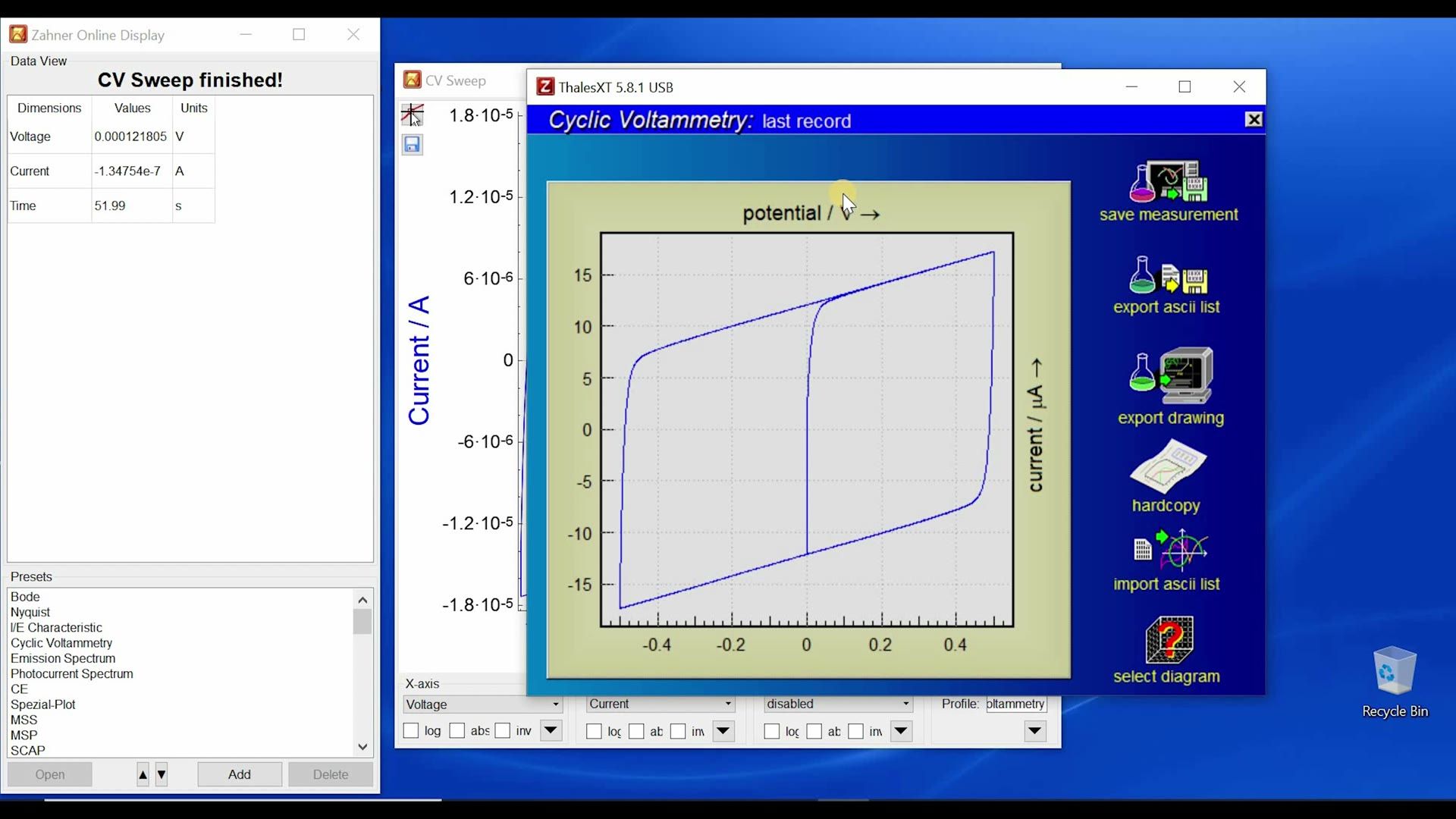
Hello everyone and welcome to this video of Zahner. My name is Waqas Saddique and in this video we are going to talk about the cyclic voltammetry and how you can set up a cyclic voltammetry measurement. For this we will hover our mouse on I/E, CV icon. This will open a sub window where you will choose CV icon and here in this window you can set up your CV measurement. In CV measurement we have a starting voltage, an upper voltage, low voltage and end voltage. So I will go for today with the default values but you can choose whatever the voltage you want to have. Here you can put a value as 0.5 volt or you can write 500M.
So both are accepted and M stands for milli. Then you have some start time and hold time. So these are the measurement times before or after measurement. So you can decide to hold at the start voltage before the CV starts and also decide to hold at the end voltage after the CV measurements are done. Here we have slew rate. So you can have positive slew rate where the software will then go from 0 to upper voltage first and you can see here the scan and then it goes to the lower voltage of -0.5 volt. But if I put in this scan - so -100mV/s then it will go from the starting to the lower and then it will go to the upper value. So you can define in which direction you want to go. For today we will just stick to the positive scan rate or slew rate values and afterwards you can define how many cycles you want to have for your CV measurement. For today let's go with 2 cycles and these are shown here. Also the measurement time is shown here. You can also define how many samples per cycle you want to have. So if you have very slow slew rate then you should have higher samples per cycle. So for today I can go to for example 2000 samples per cycle and if you are not sure how many samples per cycle you should have for your own CV scan where you have a different voltage range and a different slew rate just go to sample per cycle, right click with your mouse and this will open the PDF and here you can see a formula. So here you can give your cycle voltage span. So I am going from minus 500 mV to plus 500 mV so that is 1 V. How many samples per cycle you want to have and how many slew rates you have so you have sampling rate.
And you can define 3 values and 4th value will be given to you by this formula. So this way you can properly set up all the parameters here and then you can do your measurement. Like our I/E software here you also have option to do ohmic drop correction. So if you put a star here and click ok the system will measure the series resistance and here I have a series resistance of 10.1 ohm. As I said in my previous video that when you are doing ohmic drop correction then as a general rule of thumb take the 90% value of whatever comes up. So I have 10 so I will take 90% that is 9 ohm. Click ok and then you can do the measurement. If we put here 0 the ohmic drop correction will be automatically deactivated.
Now for today we want to go from 0 to 500 mV and minus 500 mV. Let's say I have a new sample and I don't really know how high the currents will be at 500 mV and minus 500 mV. So the one option is that I go to control potentiostat and I give here for example 500 volt and then turn it on and see how high the current would be. And then I can choose an appropriate current range but if I expect some current peaks within my CV then this option is not very suitable.
And for this we have this overflow and underflow restart and you just select this both on and just start recording. We have the highest current range which is selected and now the potentiostat will do a scan so we start from 0 we went to 0.5 volt and now we will go to minus 0.5 volt and the potentiostat will see the currents are very small but our axis is very large and it will automatically change the shunt resistance within the potentiostat and now you see that the y axis is minus 5 to plus 5 mA.
Again the potentiostat make a scan from the starting value to higher potential and lower potential so it goes to the whole scan range to see that what are the current for the whole scan range. If the currents are too low it will optimize the current range for you and once it finds the appropriate current range where it measures the sufficient current then it start recording your CV scan. So now you see it will not stop here but it will keep on measuring the CV scan. I will just skip to the end of this scan to save some time. The scan is finished and now we can save the scan. Now here you can check also that your scan is within the range of plus minus 20 micro ampere. Now you can here provide appropriate current range so minus 20 micro so micro would be with you with 20 micro and now you can deactivate this and by deactivating this now the potentiostat will not actively look for the appropriate current ranges and will follow your current ranges. If for some reason you did not set your current range properly and during the measurement the current exceed this current range the measurement will stop. So that's why it's better to have some room between your highest current and the current range which you have decided on. Another very important thing is that if you are working with very very slow slew rate so for example I am working with 100 micro volt per second now the whole measurement will take 13 hours or 14 hours.
If I do not provide the appropriate current ranges I just want to use the overflow and underflow restart and here I have minus 3 ampere to plus 3 ampere current range then it will take the potentiostat very long to validate the correct current range it may last up to hours. So if you are working with slower slew rates then it is better to first get an idea about the current range and set the appropriate current range and then deselect these two. So with this we came to end of this video I showed you that how you can set different parameter for your CV measurement. In the next video we will start with the impedance spectroscopy so thank you for your time and see you in the next video.
Einführung in Strom-Spannungs-Messung (I/E) ()
Textfassung: Einführung in Strom-Spannungs-Messung (I/E)
Automatische Abschrift
Hello everyone and welcome to this video of Zahner, this is Waqas Saddique. Today in this video, we are going to talk about the I/E scans. For this, we will hover our mouse on I/E, CV icon and this will open the sub-icons and here we will choose I/E icon. Here we can measure the current voltage curves. As you can see here that we can follow a general voltage behavior. For example, I can go from 0 to 500, then I can come back to -100 and then I can go back again to 100.
So it is up to you how you want to change the voltage. If you want to measure I/E curve only between two data points, then you can set the third and fourth data point the same value as the second one. And this will then move these values and you will have only two data points. Okay, now if we look here, we have scan mode button and when you click on scan mode, you have three different options of scan. Steady state sampling, fixed sampling and dynamic scan. Now to understand these, we have to look how a machine, how a potentiostat apply a voltage.
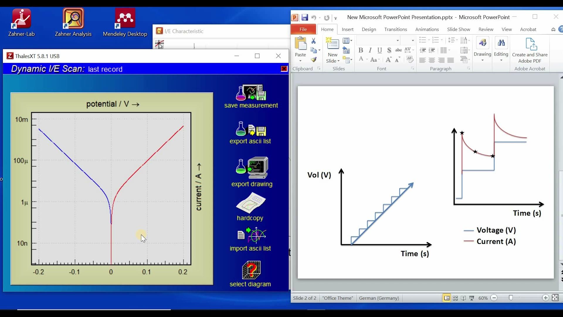
Here I have a voltage curve. So we are going from one voltage value to another voltage value. So this is the linear voltage change with time. Now when we define in a software that go from 0 to 500 millivolt for example, do the potentiostat change the voltage analogically? Do the potentiostat change this voltage with small steps? So do we have this straight line or do we change the voltage in small steps? Well in this digital world, potentiostat use the second option where the voltage change occur in small steps.
And now here I am showing very big steps when in reality they are small steps. So you can have few micro volt per steps. Now let's look at these steps in detail. So when I go from one voltage, so let's say this was your voltage and this is 20 micro volt. So when I go from 0 in no time to 20, how does the current change? Well as soon as I increase the voltage, I see a very sharp current peak and then with time the current starts to decrease.
And then comes the time when the current somewhat stabilizes and then with the next step we have another peak. Now we should ask ourselves one question. Where should we measure the current? I have here three sample data points marked with stars. Depending upon which current measurement I take, I can have different kind of current voltage curves. And this thing we can define here in the scan mode that where you want to measure your current value. So the easiest of these three options is fixed sampling. So let's start with that.
In fixed sampling you just define a time after which the measurement should be done. So for example here default value is one second. That means the potentiostat will increase the voltage and wait for one second and then see whatever the current value it is. It will record that, make the next step, wait one second, whatever the current value is recorded and so on and so forth. So this is the easiest thing. And here the voltage step is defined by this value. So here you can also make very small steps.
Now the second mode is steady state sampling and as the name suggests you can define the steady state in your sample. So for example when we apply the voltage we have this huge current and now the current is changing very fast. We are not in steady state and after some time the current changes very less and you can define that here. So default value is one nanoampere. That means when the current change is less than one nanoampere per second then take the value. You can give here one milliampere, one microampere.
Whatever is steady state for your sample you can define this absolute value here or you can define this value in percentage. To understand more about these data points just right click with your mouse on these data points. And this will automatically open the IE manual where these values are properly defined. So you have an absolute and a relative current tolerance and this defines where the current measurement is taken. Now it could also be that you were very optimistic by defining these values and then this value will never reach.
Your current change is always higher than your defined threshold. In this case we use this maximum time delay. So if after this maximum time the tolerance is not reached the system will take a measurement and move to the next step. So this is the second mode that is the steady state sampling. With the steady state sampling by giving a current tolerance value you are mostly measuring your current in this range. And with this you ensure that you are measuring faradaic response and this non-faradaic response is not measured.
The third option is dynamic scan. And in this dynamic scan what the potentiostat basically does is that it integrates the whole peak and it measures the whole current under the curve. So you just define your scan rate as we were doing with linear scan in the last video in polarization and you define your voltage values where you want to go and then you can start your measurement. Now here if you know what are the current ranges for your samples. For example if you know that from 0 to 500 millivolt your current will not increase more than 1 milliampere then you can put here the appropriate current ranges.
Last but not least we have here the ohmic drop correction. So if you have series resistance in your system you have high electrolyte resistance you can remove the effect of this additional resistance from your IE scan. If you know your series resistance just put it here if you don't know this click on this data box and then insert a star and click OK. And with this the potentiostat will measure the series resistance for your sample. As a general rule of thumb you should give here 90 percent of the total resistance.
So I have 10 so I will put 9 ohm and then I will click OK and with this you can start your measurement and the ohmic effect will be removed from your IE curve. When you activate the ohmic drop correction this correction is not done in your measurement data by the software but actually done by the potentiostat with the analog positive feedback loop. So now we have defined our voltage values and you can also choose an appropriate scan mode and then you can choose if you want to have an ohmic drop correction or not.
If you don't want to have it just click here and provide zero and then the ohmic drop correction is deactivated. So after defining everything you can click on start recording and you will start the measurement. Now I have set the parameters for a sample measurements and I am going to carry out a measurement from minus 200 millivolt to 200 millivolt. The scan mode which I have decided to do today is dynamic scan with a scan rate of 10 millivolt per second. I am not going to do ohmic drop correction and as a dummy sample I am using my test box with low Z setting.
So with this let's start the recording. So we start from minus 0.2 volt. The one thing which you should note here is that the Y axis is a log scale and to save time I will just skip to the end of this measurement. Okay now the measurement is just finished and you see here that we have very nice IE curve. So you can save the measurement I will not do it for today and with this we come to the end of this video. So I showed you today that with IE option you can have different kind of scans.
So we have we offer three different options and by choosing different option you can define if you want to have your IE measurement only with the faraday corresponds or faraday or non faraday corresponds. So with this I thank you for your time and I will see you in the next video.
Einführung in elektrochemische Impedanzspektroskopie (Teil I) ()
Textfassung: Einführung in elektrochemische Impedanzspektroskopie (Teil I)
Automatische Abschrift
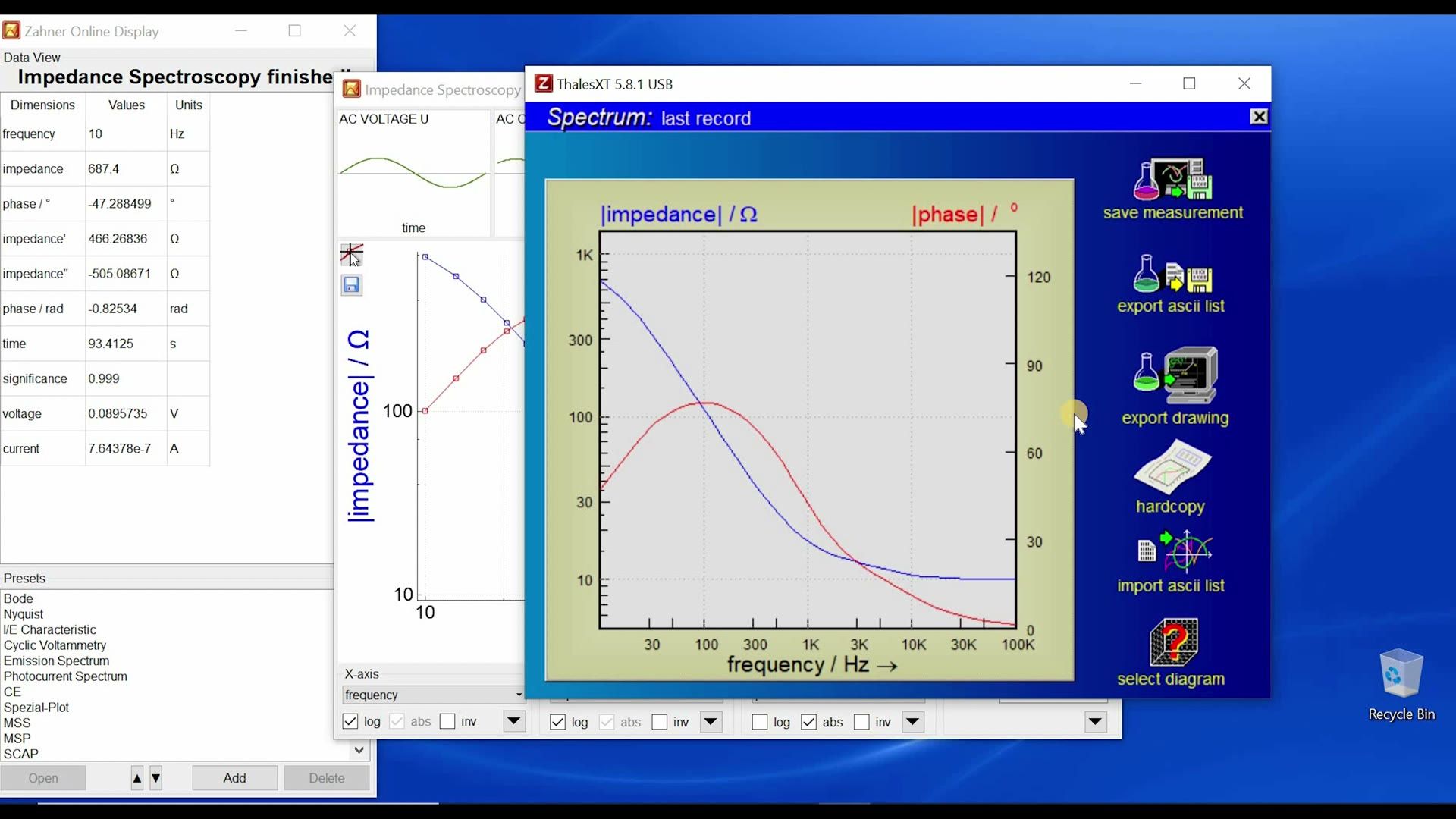
Hello everyone, and welcome to this video of Zahner. This is Waqas Saddique. Today we are going to talk about the impedance spectroscopy and how you can set up the impedance spectroscopy measurement in the Thales software. For this, we will click on this EIS icon and we landed in electrochemical impedance spectroscopy EIS window. Now here, you can set your desired frequency range. So I'm going with 10 Hz to 100 kHz, the lower and upper limit. Then you can define step per decades for the lower frequencies and higher frequencies. So for higher frequencies, we have chosen a limit of 66 Hz because above 66 Hz, the measurements are taking very less time. So you can have relatively higher numbers and at lower frequency values. So below 66 Hz, you choose relatively less steps per decades or less measure periods because the time for the measurement will increase very fast. Okay, so we can go to control potentiostat and in control potentiostat, we can set our bias voltage. So maybe I want to do a measurement at 0.1 V. So I will do 0.1 V and then I can turn on my potentiostat.
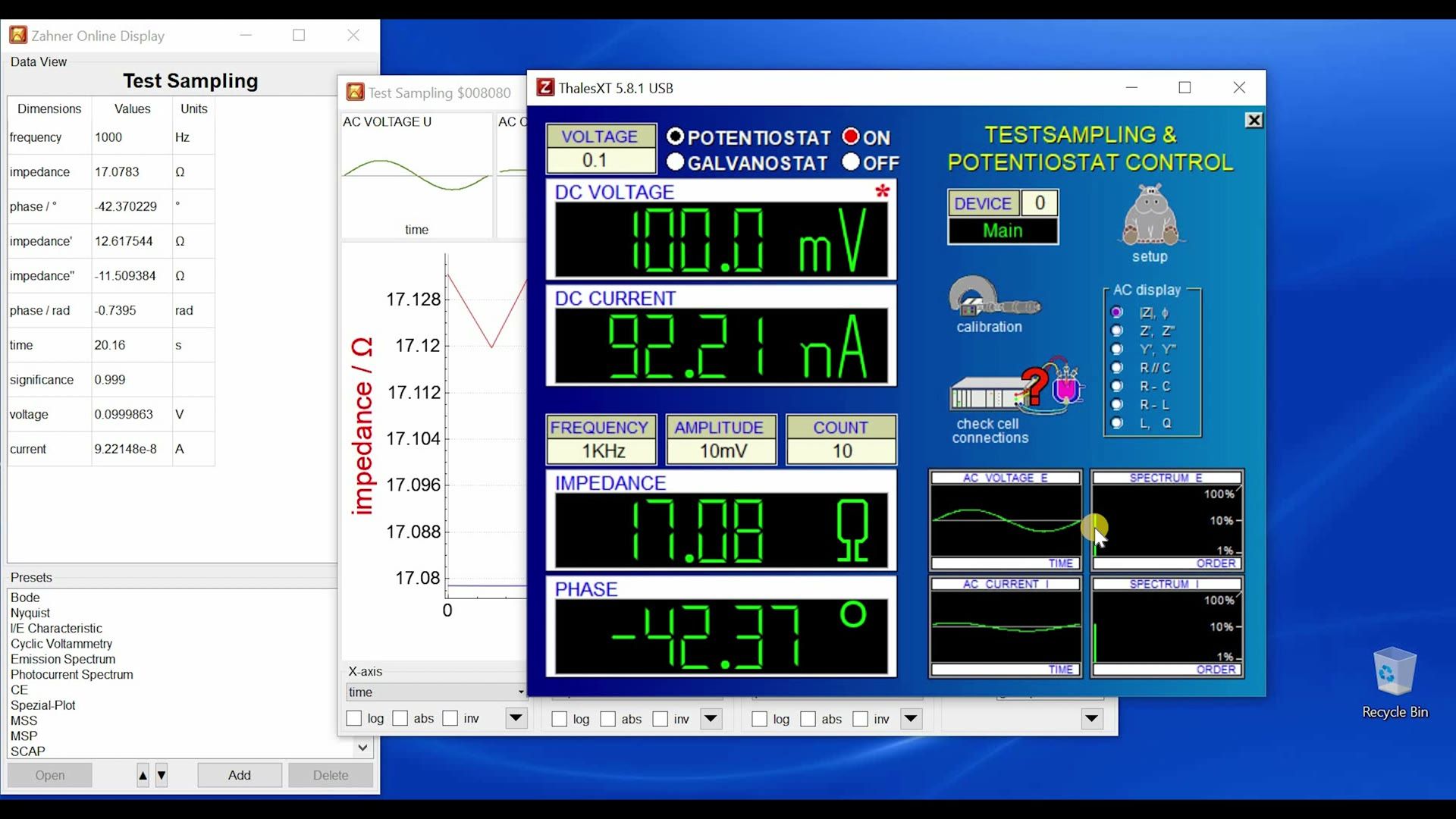
So I'm applying 100 mV and now I can set an amplitude of 10 mV and by applying the amplitude of 10 mV, we see here the impedance and phase. So you see these two values because here we have selected the impedance and phase. If you select a second value, then you will see real and imaginary impedance. Okay, now a very interesting thing is these four windows. So the upper one is AC voltage E. So this is the sine wave of the voltage signal with the 10 mV excitation and this is the response of current.
This is also a sine wave and these two windows are the Fourier transform of these two windows respectively. That means here we are looking at the time domain and here we are looking at the frequency domain. So this tells me that if I have one single line here and here, that means we are in the linear range. So we do not have to modify our amplitude. Let's say that if your amplitude is very high and you see here a sine wave, but in your response you save more than one line here, then you have to decrease your amplitude. Now, if I turn off this measurement, I can go to Galvanostat and for this measurement, I will choose the low Z setting on my test box, which I'm using as a dummy sample and for the low Z in Galvanostat mode, I will put here 125 mA as the DC bias, turn it on and now I can give an amplitude. And if I give a very small amplitude, let's say 100 nano ampere, you see that my amplitude is very, very small. I do not see any signal here. So you have to increase your amplitude because if you do not see a line here in the Fourier transform window, that means your amplitude is very small. So let's increase it. Now I will go to 1 mA and you see that we have some response. So here is your excitation signal now and the voltage is your response signal. Of course, 1 mA is also very less. So if I go to 10 mA, I should have sufficiently high signal. So 10 mA over 125 mA DC current is a good value for this kind of sample. But if I give higher excitations, for example, if I go to 100 mA, I see now that my excitation signal, which is the current value is one line, but my response is not signed. So this looks a bit distorted. And if we look at the Fourier transform, we see that we are not in linear range, but we are also getting the high frequency response. And this is because the nonlinearity in our system. Well, as a general rule of thumb, if you see such a behavior, if you see such lines, what you have to do is that you have to decrease your amplitude.
So what I'm doing here is I'm going a bit too extreme, just to give you guys an idea that how to properly select the amplitude for different bias voltage or different bias current. However, you want to do your impedance measurement. Once you have selected a good enough amplitude where the both lines are single lines, you can just go back and now I can start my measurement. But before I start my measurement, I'm going from 1 kilohertz to 100 kilohertz, and then I'm going back. So you have chosen here this pattern. So I'm going from middle to higher and then to the lower value. We can also go from middle to the lower and to the higher value. But if we do that, then we are doing double measurements at the lower frequency and the time of the measurement will be very long. So that's why a common practice is start from the center, go to the higher frequency and then go to the lower frequency. Why do we do that? I will show it to you. So I start the measurement.
One thing which I also have to note down here is that for each measurement, we are showing you the Fourier transform. So anywhere you see more than one line, you know that you have to decrease your amplitude. Now we start from the center. We are going to the higher frequencies and then we will go back to the lower frequencies. A condition for impedance spectroscopy is stationarity. That means your system should be stable. If it is not stable, if it is not stationary, the data which you are getting when you are going from the middle frequency to higher frequency would be different than the data which you will decode when you are going from the higher frequency to backwards. And if these data are not overlapping, you know that your system is not stable. And if it is not stable at this high frequencies, it will not be stable at lower frequencies and then you will not get good results. So this kind of hint, if your sample is good enough for this measurement or if it is too unstable. And here we can see that it is good enough the data is overlapping perfectly.
So we can trust this impedance measurement. And now we are at the end of the measurement. And with this, we are finished with the measurement. We have the impedance data and we have the phase data. You can save this measurement. I will not save this measurement. Now we have done this measurement at constant current in galvanostatic mode. So the potentiostat is on and we have to turn it off after the measurement. So with this, we came to the end of this video. I showed you that how you can do an impedance measurement.
What is the function of these windows where you see the Fourier response, which helps you in choosing a suitable amplitude Fourier measurement and also what is the function of this double measurement where you are starting from the center and you are going to the upper frequency and the lower frequency. In the next video, we will continue with impedance spectroscopy. So today we did a measurement in galvanostatic mode. Similarly, we can do a measurement in potentiostatic mode and open circuit and pseudo galvanostatic mode. So we will talk about this in the next video. Thank you for your time and see you in the next video.
Einführung in die elektrochemische Impedanzspektroskopie (Teil II) ()
Textfassung: Einführung in die elektrochemische Impedanzspektroskopie (Teil II)
Automatische Abschrift
Hello everyone, and welcome to the second video of electrochemical impedance spectroscopy. This is Waqas Saddique. In my last video, we did a measurement in galvanostatic mode, where we have a bias current of 125 milliampere and amplitude of 10 milliampere. Now, if you click on amplitude, on the top of this data box, you can see that you can either put the value in ampere, so you can have 1 picoampere to 2.88 ampere, or you can have your value in volts. So if I put here 10 millivolt, now I am in pseudo-galvanostatic mode, where my excitation is in millivolt, but my bias current is in current.
So when we turn it on. So now here, we have our bias current, and on this bias current value, we have our excitation in millivolts. Now if we look in the Fourier transform window, we have two lines for our current value. And this tells us that we are in the non-linear range. And therefore, we have to decrease our amplitude. So I will click on amplitude, and I will put here 1 milli. Don't forget to put here volt, otherwise if you put just 1 milli, it will go to 1 milli ampere.
And with 1 milli volt, we can see that both the excitation and the response are showing us one line, and this way we can do a pseudo-galvanostatic impedance measurement. An important thing when you are using the test sampling window is that when the measurement is going on, then make sure that your cursor is not on any active button. So for example, here, if I move my cursor above count, then you will not hear this ticking sound which comes when you are doing impedance measurement. And then it could happen that here, in the impedance and phase, you will see some random values.
But if I remove the cursor, now you will start hearing this ticking sound again, and the measurement will start again. So in the test sampling window, when you come on any data field, the software assumes that you are going to change some value, and then it will stop the measurement. So keep this in mind that when you are testing your sample in the test sampling window, then you do not hover your cursor on any active button. Okay, so we talked about Galvanostat in the last video.
Now we talked about pseudo-galvanostatic mode. We can turn this off, and we can go to potentiostat, and in potentiostatic mode, you can give your bias voltage and the amplitude in volts. Now let's say that I put 0.1 volt, and here I have 10 millivolt, and I turn on my potentiostat. Here I have excitation and response signal in the Fourier transform IC1 line, so my amplitude is good enough. Now if I will go back and start that recording, I will do an impedance measurement with potentiostatic mode.
So I will do the measurement with the bias voltage of 0.1 volt. But if I just turn off my potentiostat, so I turned off my potentiostat, and now keeping the potentiostat off, I go back, and then if I just start recording the measurement, I will now do the measurement at open circuit voltage. So the software will now measure the open circuit voltage and keep this voltage as our bias voltage, and do the measurement with 10 millivolt amplitude. So again here, we start from the center frequencies, 1 kilohertz, we are going to the higher frequency, and then we will go back to the lower frequency.
For this measurement, I took the exp, the exponential setting on my test box. And you can see here that going to the higher frequency and coming back, the data is overlapping, so this tells me that my system is stable enough. Now I will skip to the end of this measurement to save some time. So we are finished with our measurement, we can save the measurement, but I will not do this, and I will just go back. Okay, so this is how you can do impedance measurement on open circuit voltage.
Coming back to the test sampling window, when we say that the amplitude is 10 millivolt, then this is the amplitude from 0 to peak, so that is 10 millivolt. But if we consider from peak to peak, that would be 20 millivolt. And with this, we came to the end of the second part of our impedance spectroscopy video. I showed you that we cannot only do galvanostatic impedance spectroscopy, but also potentiostatic impedance spectroscopy or pseudo galvanostatic impedance spectroscopy. And you can also do an impedance spectroscopy at open circuit potential, if you keep your potentiostat off and just start your impedance measurement.
So with this, I thank you for your time and I will see you in the next video.
Einführung in den Thales-XT-Modus ()
Textfassung: Einführung in den Thales-XT-Modus
Automatische Abschrift
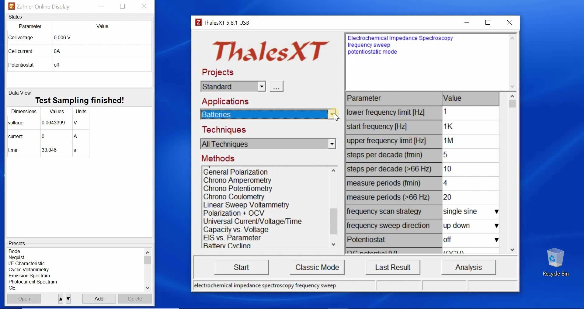
Hello everyone and welcome to this video of Zahner. This is Waqas Saddique and in this video I'm going to introduce you to the second interface of Thales software that is the Thales XT interface. This is a very user-friendly interface and is designed for the users who are new to electrochemistry so that they can easily set up and carry out different electrochemical measurements. Now having said that there are some restrictions in this interface for example there are some techniques for which you have to go to classic mode for example you cannot access your control potentiostat as we did in classic mode but if you want to do simple measurement like impedance spectroscopy or current voltage curves or cyclic voltammetry that can be easily done here. Now if we start from the top you can decide which fields you are working with so if you're working with the field of batteries then all the techniques which are related to the batteries will come or if you are working in the field of photo electrochemistry then all the techniques which are coming with the photo electrochemistry will come but in most of the photo electrochemical techniques we made this restriction that here the user have to go to the classic mode. Having said that so let's choose batteries as an example and then you can further categorize if you want to do ac measurement or dc measurement so if you want to do dc measurements for example current voltage measurements then you can also choose that and if you want to do ac measurements you can also choose that so impedance spectroscopy and so forth. Now I choose here potentiostatic mode I can give again the lower frequency the starting frequency the upper frequency the steps per decade for the lower frequency value and steps per decade for higher frequency values so on and so forth if the values are good enough they will be marked in blue so you can choose if you want to have single sine measurement or multi-sine measurements and for easiness we will stay with the single sine measurement and you can define the sweep direction so up down or down up whatever you want to have if potentiostat stays off you will do the measurement at open circuit voltage and if you keep it on then you have to tell at what voltage you want to do your measurement so I can put 100 m and then if it is good enough it will turn blue and then here you define your amplitude in millivolt once you are done you can just click start and your measurement will start and now you are looking at the Fourier transform of the excitation and response signal I will just skip this measurement to the end so that we save some time it's done and now you can click on the save icon to save your measurement you can here write any comments which you want to have and then click okay and then you can save wherever you want to save your file I will not do this for today so with this way you can very easily define what kind of measurements you want to have now here we have different kind of projects so for example in one project you are working with a frequency range where you are going let's say here to the upper frequency of one megahertz but in some other project you are working with some other frequency range and when you are working with different samples you have to always change the frequency range well that's not the case you can here put more projects so I just put here a Zahner project you can click on these three dots to make a new project or delete an existing project so if you go to Zahner you can see here that the values which are set for this Zahner project are here so for my standard project I had the upper frequency of one megahertz but for this Zahner project I have upper frequency of 10 kilohertz so you can have different projects where you have different values for your measurements and if more than one users are working then you can assign different projects to users so if more than one user are using the potentiostat then they don't have to modify the parameters for their measurement each of them can have different project and then they can just go to their project and the values which they used last time would be saved with this we came to the end of our video the Thales XT interface is designed for the easy use of the potentiostat although it's user-friendly there are some limitations to its full use and if you want to really control each and every parameter and you want to look in depth how you are carrying out the measurement then we always recommend to use the classic mode for this and that you can do by clicking on this Z icon and then switch to classic mode so with this I thank you for your time and I will see you in the next video
Zahner-Analysis-Videos
Zahner Analysis - Einführung ()
test. Try uploading the videoTextfassung: Zahner Analysis - Einführung
test. Try uploading the video
Automatische Abschrift
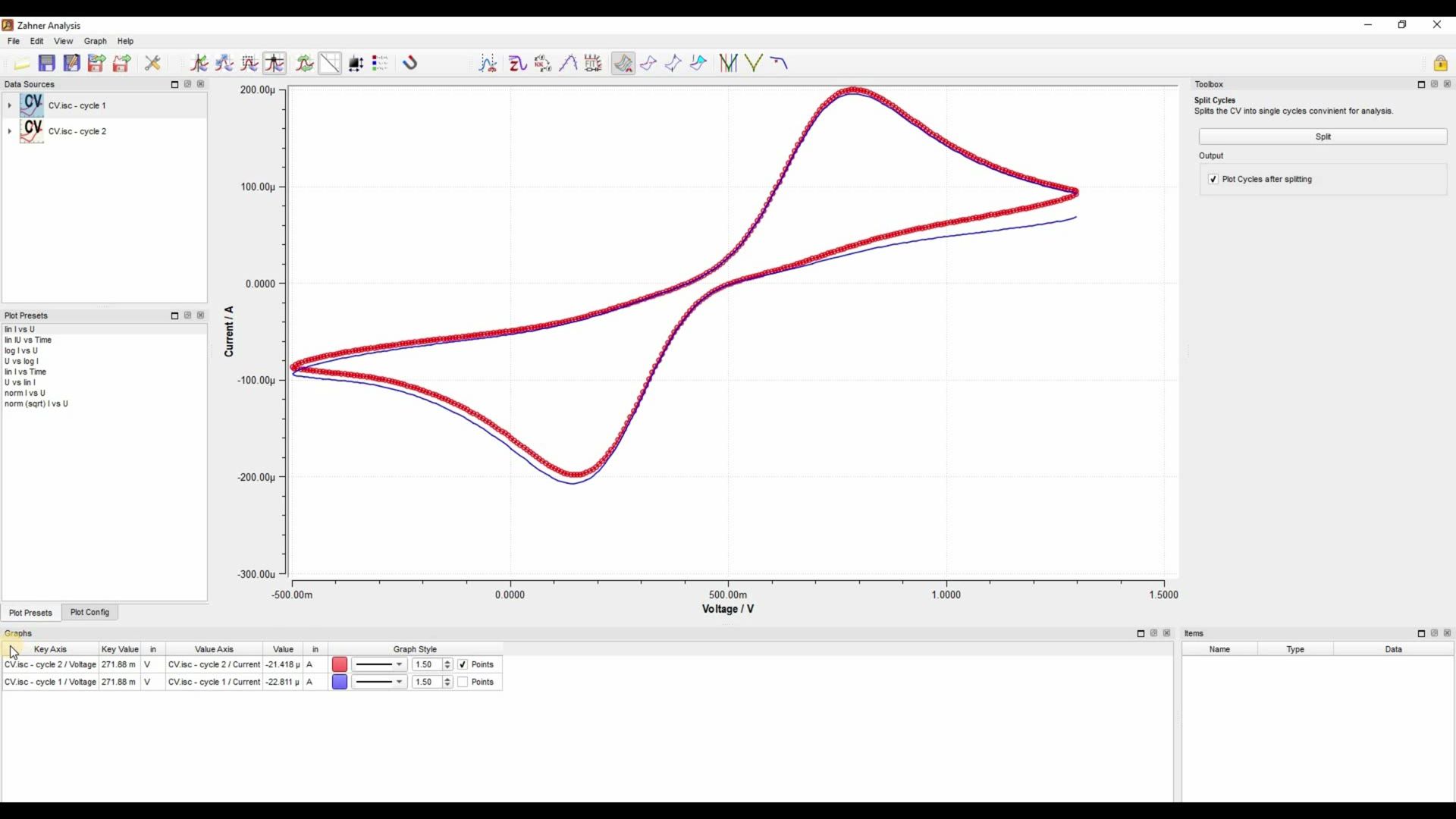
Hello and welcome to another video of Zahner. This is Waqas Saddique. I am an application specialist and marketing manager here in Zahner. In this video, I am going to introduce you to the layout of the Zahner Analysis software. So, let's get started. First of all, at the top left, we have a general layout containing menu bar and tool bar. In menu bar, we have file and edit menu and so on. And in the tool bar, we have different icons. We have icon for opening a file for saving the file to export in another format and the settings.
And then we have these two icons. These icons allow me to control my graph area. For example, the first icon allow me to produce a cursor or a label in my graph area. With the second icon, I can move my graph. With the third icon, which is the zoom icon, I can zoom into some part of my graph. And if I want to go back, I go to reset scaling. And now I'm back. The fourth icon allow me to read the x-axis and y-axis value at any point of my graph.
These five icons we used in most of our work with the Zahner Analysis software. I will introduce you to the rest of this tool icon in the later videos. Here in evaluation bar, we have different icons, which allow us to characterize our impedance spectra, your cyclic voltammogram, your current potential curves, your Tafel slope. If you have characterized the solar cell and you want to measure the maximum power and fill factor, you can do that here. And I will discuss them in detail in other videos. In this video, we are going to stick to the layout. First of all, here on the left side, we have a data source window. In this window, we see how many files are open in Zahner Analysis software. Right now two files are open. I can see one cyclic voltammogram. If I want to see the both windows, then I can go to the second graph and click on it and drag it to the graph area. And now I have my second graph, which is also red. So I can change the color. And now I have a two graphs.
The area which I just used is this area, which shows me my graphs here. You can change the color of your graphs, which are in the graph area. You can give them points in spite of lines or lines with points. You can change the size of your line. You can make it thicker or thinner. You can also click on a graph and then click delete on your keyboard and then the graph is gone. The next is plot preset. In plot preset, there are different options. There are different ways that you can see your graph. Right now we have a linear voltage linear current graph. You can change it. You can see it voltage and current versus time.
You can go to log of current versus voltage and so on and so forth. In plot preset, we have two settings, plot presets and plot configuration. Here also, you can change the way you want to have your graph. The log values, you can have the inversion values and you can have the absolute values. So you can change them for any of x-axis or y-axis. Next, if you go to this toolbar and then you right click with your mouse and go to the data view, you can see the data of your graph. If you have some artifact in your graph, let's say for example here, you do not have 1.2, but 2 volts. Now there is one point, which is here and you want to remove this, right click with your mouse and then delete. And this way, if there is some artifact, let's say within here in your graph, you can eliminate them.
Okay, that's one thing. Now we come to the toolbox window. This toolbox window you use when you are using these evaluation icons. So for example, if I want to draw a baseline, then I have to go to new baseline and then I can draw with my mouse a baseline. And this way, the toolbox gives you a window where you can use the parameters for the customization of different things here. Another example, if you want to measure the area under a peak, then you click on the integrated charge. And now in the toolbox, there is further information which you have to provide to complete the integrated charge characterization. So toolbox is a window which you use to characterize your graph. Last but not least, I draw a baseline and this baseline is shown here. If I have some cursor, that cursor will also be shown here. Or if I have a label, that label will also be shown here. I can change the name of the label. So this was a very basic overview of the Zahner Analysis layout. I tried to show you that what different part of the Zahner Analysis window do.
In future videos, I will talk more in detail about the Zahner Analysis software, what we could do with the Zahner Analysis software and more specifically, how we use and when we use these icons, which are the heart of this Zahner Analysis software. So with this, I thank you for your attention and see you in the next video.
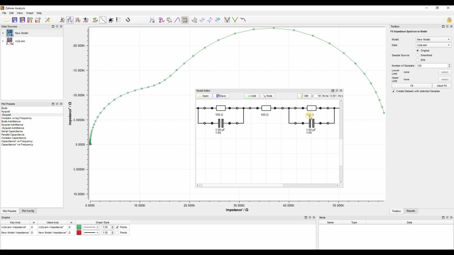
Fitting eines Impedanzspektrums ()
Textfassung: Fitting eines Impedanzspektrums
Automatische Abschrift
Hello everyone and welcome to another video of Zahner. This is Waqas Saddique. I am an application specialist and marketing manager here in Zahner. Today I am going to show you how you can fit your impedance spectra. First of all go ahead and open the impedance spectra which you want to fit. Here I have already opened an impedance spectra for me. What you see in front of you is a Bode representation where you have impedance and phase versus frequency. Since most of the researchers are familiar with the Nyquist preset. So let's go to the minus Nyquist and here you have your Nyquist graph. Now we want to fit this graph. So for this let's get started. Click on the fit EIS.
The fit EIS open a new window and now here we have to design our electrical circuit. Before you design your electrical circuit you have to have insight into your system. You should know that what is your system composed of and once you have the knowledge about your system then you can draw a true representation of your system. In my case here I have a pretty good idea that what electrical circuit can represent this system. So with this let's get started. I know that I have two electrodes so I will make an R, a resistor and a constant phase element circuit for the first electrode and then a connecting resistance and then I will have another R and constant phase element. So resistor and constant phase element for my second electrode and let's connect everything together. Now if you have a bit complex electrical circuit like I have here then this looks very messy. So what you do is that you right click with your mouse and then you click auto align and this auto align your electrical circuit in a very nice representation. Okay so now I have my electrical circuit. I have to provide here the frequency ranges. Right now 1 mHz to 1 mHz is given which is good enough for me so I will work with this but if you have to change your values just go ahead and change them now and then you click simulate and as you will click simulate it will produce a simulation file here. So let's click simulate it produced a new model here. You have to drag this model into this graph area because otherwise you will not see it here.
Right now you can't see it here but if I change the color you see that your graph is somewhere here. So before there was light blue color and it was not really visible. So just to show you that it has been drawn but since the resistances are very small that's why your semicircles in your Nyquist plots are very small. Now what you have to do is that you go ahead in your toolbox and click fit. Here we have three options original smooth hit and Z-HIT. You use Z-HIT if there are some artifacts but right now we are just going to fit with the original setting. So I click fit and you see that it started fitting the spectra. Now the software sometimes requires a bit of the time to fit and as you can see that it's changing the values here. Okay now the spectra is completely fitted. We have our values and you see that the fitting is quite good. We can go to the results here and we see that the overall error in our fitting is 0.09%. So it's a pretty good fit. Now let's see what else is provided in the results window.
Here we have each element which we have used in our fitting. We have their values. We have their significance. Significance tells us that how important this element is for this fitting. So you can see that the first resistance is this one 14.9 kilo ohm has a significance of 50.547 out of 1. It has an error of 0.26%. This resistance of 476 nano ohm is a very small resistance. So if we remove this resistance it will not change our fitting that much and you can see here that the significance is very very less.
So if you remove this resistance it does not really matter. Another very important thing is that you don't only have access to the significance numbers but you also have access to significance plot. What isn't significance plot? Well let me show it to you. You go to your model, right click and click on the significance plot and it has shown here your significance plot. Of course the y axis is too huge so we have to just change it. So I will change it to from minus 1 to let's say 7 and here is your significance plot. Let me bring this here. Now what you see here is that for example your first resistance which is 14.9 kilo ohm in which frequency range it gets important.
Another significance plot which shows you that which element is significant at different frequencies. So this is also very nice feature of the Zahner Analysis software. Now you want to export your data. So you just go to the model which you want to export and then you click file and text export. So with this you will have your text file or you can just save this fitting in your Zahner Analysis software. With this we came to the end of our video. I thank you for your attention and see you in the next video.
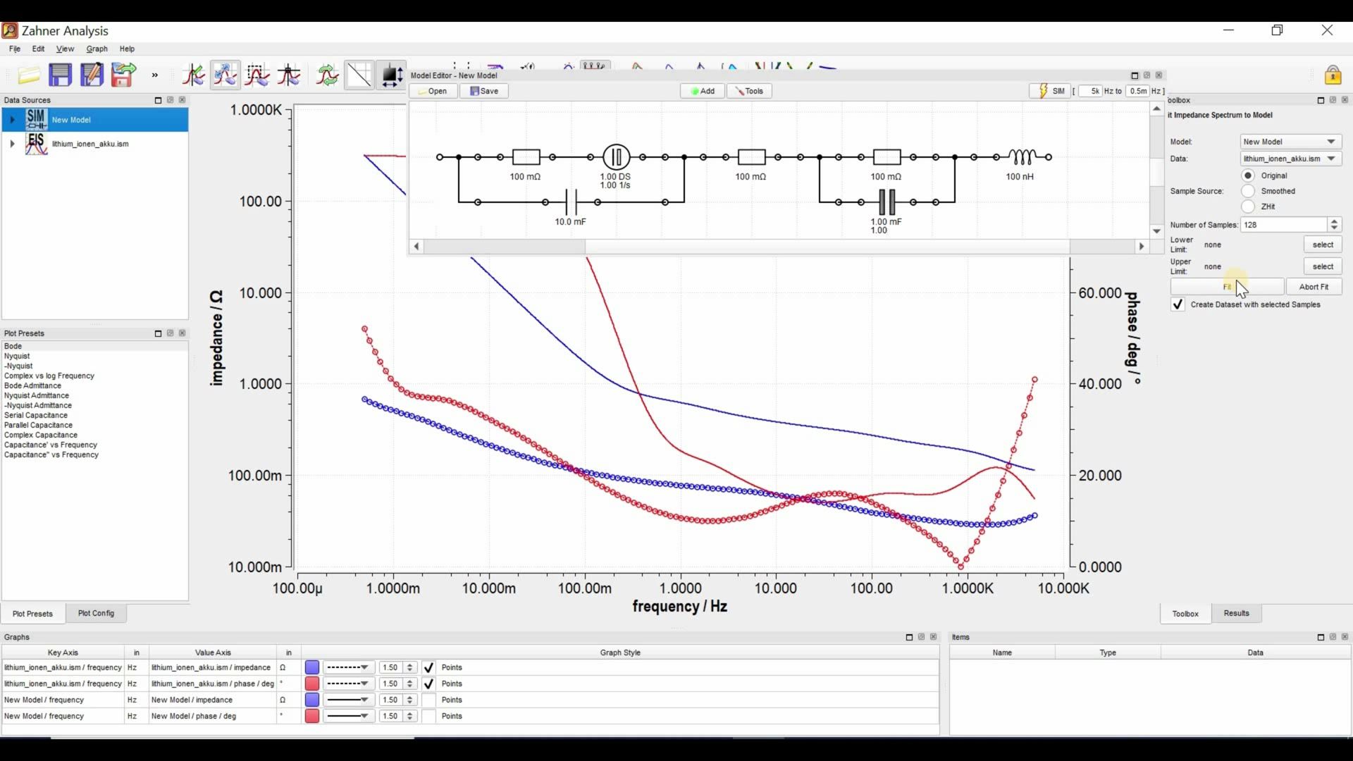
Fitting eines komplexen Impedanzspektrums ()
Textfassung: Fitting eines komplexen Impedanzspektrums
Automatische Abschrift
Hello everyone and welcome to another video of Zahner. This is Waqas Saddique. I'm an application specialist and marketing manager here in Zahner. In this video I'm going to fit a complex impedance spectra for you. I have already made a video where I fit a simple impedance spectra. If you haven't watched that video, I will suggest you to go watch that video first and then come back to this video. I will put the link of the first video in the description of this video. If you have already watched the video then let's start with the fitting of this impedance spectra. First of all we will click on fit and this opens up a new window where we will make our model. I have stretched the window so that we can see the complete model. As I told you already that we have to have insight into our system. You should know that what is your system composed of and then you can make a realistic model. I have two electrodes so I have to make two resistance and phase element circuits. So two R and CPE circuits which are connected via a series resistance. I have already made one R CPE and now this is the series resistance and now I will make a second R CPE circuit. And as you can see in the Bode diagram that we have inductive behavior in our spectra so we also have to add an inductance. So here is our electrical circuit and if you remember from the last video this is the same electrical circuit which we used in the last video. But here you will see that we have a diffusion behavior at the lower frequencies.
If we go to the Nyquist we see this diffusion behavior here and such a diffusion behavior can be recreated by a finite diffusion element. So I will put this finite diffusion element next to this resistance. So here is my finite diffusion element. Now I face another problem and that problem is that this finite diffusion element is in parallel with this constant phase element. And we know that these two elements work against each other. So if now I do a fitting it will give me very bad results. So what I can do is that I can remove this constant phase element and I can replace it with a capacitor. So a tip here you cannot use a finite diffusion element with a constant phase element in parallel. Now we have our modified electrical circuit and we modified it because we have this diffusion behavior.
Let's go back to the Bode plot because there we can see the diffusion behavior and the inductance behavior. Now I can go ahead and do fitting and then I will have some fitting results. But since this electrical circuit is very complex so it's always better to give some starting values in the software so that the software can start fitting in the right direction. So I know that in my system the resistances are in milli ohm range. So I will give all the resistance a milli ohm value. You don't have to give any specific value just put the values in the milli ohm range and then it's enough. And also the capacitance I will go here in the milli ohm range. And for this constant phase element I will also go into the milli ohm range. Okay so that's good enough.
Now I can simulate and with simulation you create this new model and now I will drag this new model here. This red and blue curve is showing me the Bode results for this electrical circuit. Now when I will click fit it will start fitting the impedance spectra. And you see that because I had already given the suitable ranges it was very easy to fit the impedance spectra. If you had such a complex impedance spectra and you do not give these starting values and you just click fit you will see that you will run into problems. So it's always a good idea to give suitable starting values. And now the fitting is complete we go to results. As you can see in the result window that we have an overall error of 0.3 percent. So this is a quite a good fit. And we can see the significance and error of each element.
Another thing which I want to show you is this export if you click here in the export and you click PDF export and then you save the data in the form of a PDF. I did a PDF export for you. So here is the PDF which was saved and what you see here is that you have your spectra and then you have your fitting. It would have been better if I would have used different colors but you can see that these points are showing me my spectra and these lines are showing me my fitting. I have my electrical circuit which was used for the fitting and then I have each element their values and their significance and the error. And at the end I also have the overall error of 0.302 percent for my fitting. So this is also a nice fitting report if you are doing some fitting and you have to quickly go to your professor or your colleague and you want to show your fitting results. So I hope that in this video I was able to show you that how you fit a complex impedance spectra. Just to summarize you have to have insight into your system. You should know that what is your system composed of. You should have a realistic electrical circuit. If you know that you have inductive and diffusive behavior then you have to put relevant electrical element into your electrical circuit. It is always a good idea to give appropriate starting value and this makes your fitting very easy. If you do not do this step you will run into problems. So with this I thank you for your time and I see you in the next video.
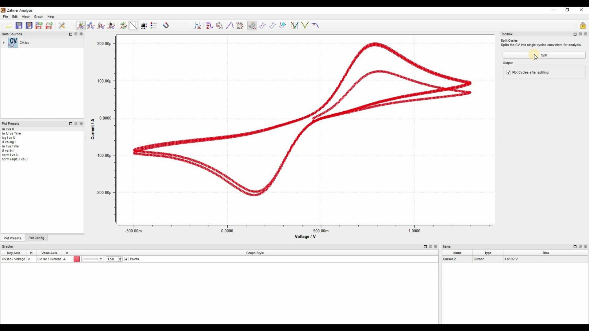
Charakterisierung eines zyklischen Voltammogramms - Teil I ()
Textfassung: Charakterisierung eines zyklischen Voltammogramms - Teil I
Automatische Abschrift
Hello and welcome to another video of Zahner. This is Waqas Saddique. I'm an application specialist and marketing manager here in Zahner. Today I'm going to show you how to characterize your cyclic voltammogram. More precisely, we are going to draw a baseline, measure peak height and integrate the area in a peak. So with this, let's get started. As you can see here that I've already opened a cyclic voltammogram. Before we start, we have to remove any artifact if present. As you can see in my cyclic voltammogram, I have an artifact. To remove this artifact, there are two possibilities. One is I can cut my graph and that you can do by clicking on the cut graph. And as I click on this cut graph icon, the further information comes up in the toolbox. Now I can cut right or the left part of my graph. I can click in the graph window with my mouse and make a new cursor here. And in the toolbox window, I can click on remove right to remove this part of the graph. So remove right and now what you see is that I have my graph here. I can go to the x-axis and drag my x-axis to the right so that the graph is in the middle. Another possibility to remove the artifact is that you access the data file of your cyclic voltammogram.
To access the data file, you right click on the bar here with your mouse and then you go to data view. And now you have your data file for your cyclic voltammogram. And here you can go to the individual point and then you can delete the selected row of your artifact. This way you can remove the individual data point within your cyclic voltammogram. Now I have my cyclic voltammogram. But this cyclic voltammogram has multiple cycles in it. For the sake of this video, I only need one cycle. So let's do split cycle. For splitting cycles, you go to split cycle and then in the toolbox window you click split. And now I have multiple cycles. Let's remove right by clicking delete on my keyboard. I have this new cyclic voltammogram.
And now the first thing which I want to do is draw a baseline. For drawing a baseline, we click on insert and edit baseline. For this cyclic voltammogram, I will draw a baseline which is parallel to the initial slope of the cyclic voltammogram. Let's draw a baseline for the anodic peak here. And your baseline is shown here in this items window. You can draw another baseline. For this, you can click on new baseline. I will draw the second baseline in accordance to the initial slope of the cathodic curve.
So something like, like this. So here you see that the initial slope is the same as baseline. The next goal which we want to do is measure the peak height. So I have chosen baseline one. And now we can go to the select peak icon and then you go to the peak position and we click there. And in the items window, we see that anodic peak position and its height, which is 202 microamps per centimeter square. Similarly, for cathodic peak, we have to choose the baseline two because that is the baseline for cathodic curve. And we go to the cathodic peak and we click with the mouse there. And now we have a cathodic peak with the position at 154 millivolts and the height of minus 184 microamps per centimeter square.
Okay. So this is how you draw a baseline and how you measure the peak height and position. For the third part of the video, I have created everything the peak positions and the baseline leaving only the baseline one. Here is our baseline and now we want to integrate the anodic peak. For this we go to Integrate Charge. In the toolbox window, you have to provide further information for integrating the peak. First of all, the baseline one is selected right now. If you have multiple baselines, for example, you have two baselines for anodic peak and the cathodic peak, then you have to choose the relative baseline for the peak which you would want to integrate. Next, you have to provide the start and end of the peak. So let's go and select for choosing the start point of the peak. I will say that my peak is starting from here. So I will click here for my start of the peak. And now for the end of the peak, you don't have to go here for the end and select and then select the peak, but it's automatically selected. So you can just click with your mouse at the end of the peak.
And now you have your start and end of the peak. Currently, the plot preset is current versus voltage. But as you click on Integrate Charge, this plot preset from current versus voltage will be changed to the plot preset of current versus time. So let's click on Integrate Charge. And here you see that the plot preset changed from current versus time. And here you have your integrated peak area. The information about the integrated peak area is provided here. You can see that we have a positive peak that is our anodic peak. It has an integrated area of 529 micro coulomb per centimeter square. We also have a negative point. Since we did not integrate our cathodic peak, so negative part of the area is zero. The software also provides you the net difference between the both peaks. So let's say if we had integrated both the anodic and cathodic peak, then the net value will show the difference between the both peak areas. So with this, we come to the end of our video. In this video, I showed you how to draw a baseline, how to measure the peak height and the peak position and how you can integrate the peak area in a cyclic voltammogram.
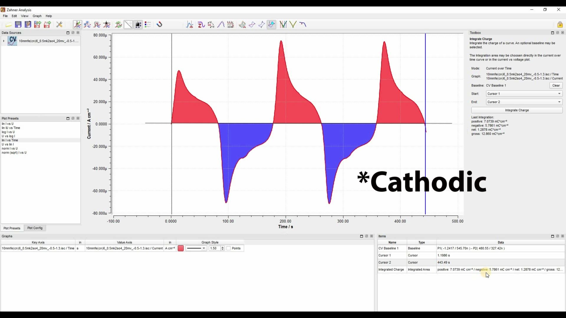
Charakterisierung eines zyklischen Voltammogramms - Teil II ()
Textfassung: Charakterisierung eines zyklischen Voltammogramms - Teil II
Automatische Abschrift
Hello everyone and welcome to another video of Zahner. This is Waqas Saddique. I'm an application specialist and marketing manager here in Zahner. In this video I'm going to talk about cyclic voltammogram. Previously I showed you that how you can draw a baseline, measure the peak height and peak positions and how you can integrate peak area. Today we want to go one step further and to analyze all the cycles of the cyclic voltammogram simultaneously. To better represent the cyclic voltammogram, this time I will choose the linear I versus time plot preset. In this plot preset I have current versus time representation and what I want to do is that I want to integrate all these oxidation peaks and these reduction peaks simultaneously. For this let's get started. First of all we have to draw a baseline. For this we go to the insert and edit baseline. I will just draw a baseline at zero front.
So this will be my baseline and now I want to integrate the charge. For this we go to integrate charge. Now in the toolbox it shows us that what we have to do we have to provide the starting point of the graph and the end point of the graph. For providing the starting point of the graph we can go to the graph, right click with our mouse and make a new cursor. This cursor one is automatically selected here and then go to the end of the graph and then make a new cursor by right clicking with your mouse.
This cursor two is automatically selected for the end of the graph and now if I integrate charge I will integrate all these oxidation and all these reduction peaks. So let's integrate charge and now all the peaks are integrated. The results are shown here. Here you can see that we have baseline over two cursor positions and here is our integrated charge. What we see here is that the three anodic peaks are shown here as positive which has the charge of 7.07 milli coulomb per centimeter square and these anodic peaks have the charge of 5.78 milli coulomb per centimeter square. It also shows the net value which is the difference between the positive and the negative value that means this is the difference between the anodic and the cathodic peak. So if you have multiple cycles and you repeat this process at the end it shows that if your material has oxidized or reduced. So this is a very nice feature of Zahner Analysis. Now allow me to introduce you to another very nice feature of Zahner Analysis.
For this we have to go back to the linear I versus U plot preset. Now go to the data sources window and click on the active file, right click go to properties. This opens up a new data set properties window. This window provides all the information which you provided during the measurement in the Thales software. Here we have the information about the system, temperature, the time it was measured, the slew rate. If you had any comment you can write your comments here. One very nice thing is that you can choose the reference electrode potential. For example right now silver/silver chloride is chosen but let's say that you were using calomel electrode. So you choose the concentration of the calomel electrode and then you click apply and you will see that this y axis will shift. Now it has adjusted your cyclic voltammogram regarding this new reference electrode.
You can also choose a user defined element and then you have to provide an offset. Here you have to decide what was the offset. If you click 0 then it will shift the whole value by the difference from the previously chosen value. In the Thales software you have the option to do the correction for the ohmic drop. If you did not do that there you can do that here. So you choose the ohmic drop resistance and then you click apply and it will do the ohmic drop correction. Another very nice thing is that you can provide the area of your electrode. Right now one centimeter is chosen.
If you choose two centimeter and you click apply this y axis will change. You see here the y axis has changed to the half of the previous values and if you go back the y axis will double than what was given before. And another very important thing is that when you are changing the area your y axis should be in amps per centimeter square. If it is in amperes you will not see the difference in y axis by changing the area. And how do you change from amps per centimeter square to amperes by clicking on this icon and if you click again you go back to amps per centimeter square. So keep this in mind that if you change the area then you have to make sure that you are in amps per centimeter square y axis setting and not only amps. So with this we came to the end of our video. In this video I showed you that how you can integrate all the peaks of your cyclic voltammogram simultaneously and how you can change the setting for the reference electrode, the ohmic drop correction and the electrode area. With this I thank you for your time and see you in the next video.
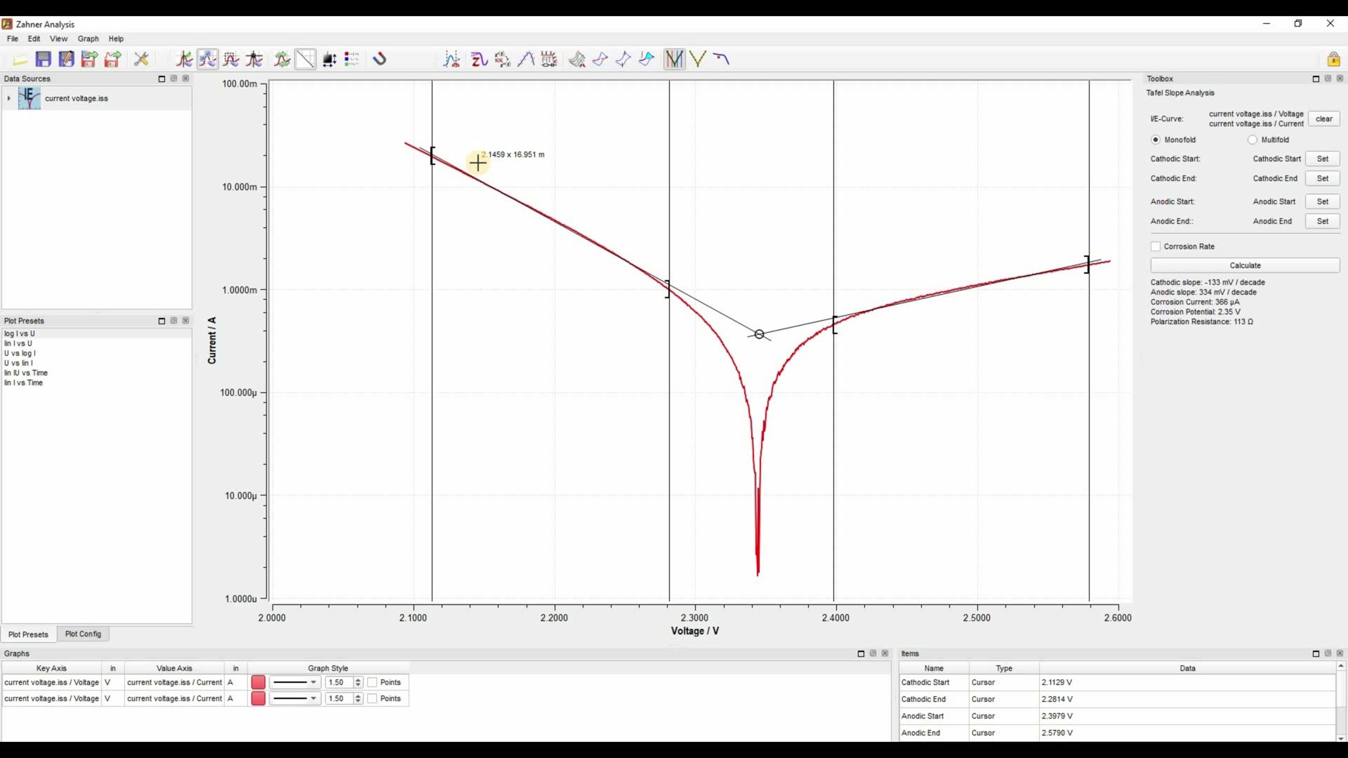
Tafel-Steigung ermitteln ()
Textfassung: Tafel-Steigung ermitteln
Automatische Abschrift
Hello everyone and welcome to another video of Zahner. This is Waqas Saddique. I'm an application specialist and marketing manager here in Zahner. Today we are going to measure the Tafel slope for an current-voltage curve. As you can see here that I have already opened a current-voltage curve and I want to measure the cathodic and anodic Tafel slope. So for this let's get started. As you will click on this Tafel slope icon you will see that in toolbox window some additional parameters are required for the Tafel slope analysis.
So first of all we need to provide cathodic start, cathodic end, anodic start and anodic end. Here I will click set to set the cathodic start. So let's click here and then you have to also give cathodic end. So you don't always have to set the set value and then go to the appropriate value. So here will be cathodic end. Next come anodic start. Let's start it here and anodic end here. Beside Tafel slope analysis you can also measure the corrosion rate but for the corrosion rate you have to know the area of your electrode, the density and the equivalent weight. We will skip this for now and then by clicking calculate it fit my Tafel slopes and it measures the Tafel slope. You can see here that the cathodic slope has a slope of 133 millivolt per decade and anodic slope has a slope of 334 millivolt per decade.
There are also some additional information given here in the window below you see cut set positions and you also see the equations for the Tafel slope and you see the point where the both slopes are meeting up. So they are these both slopes are meeting at the 2.345 volts. So here okay so this is how you measure the Tafel slopes of your current voltage curve. For the second part I will just remove this cursor. Now we want to measure the Butler-Volmer characteristics of our current voltage curve. For this we will go to the Butler-Volmer icon. Again in the toolbox there are some parameters which we have to provide. First of all we have to set the left's cursor. So then let's set it here and then the right cursor is automatically chosen. Again you don't have to set it up and then just do Butler-Volmer fit and then it shows you the fit. It also again show you the anodic and cathodic slope and in this window you see the Butler-Volmer parameter.
You see that it's not symmetric so symmetry is 0.247 effective C is 542 milli. So you can change the temperature we did not and it took the standard value of the temperature which was 298 Kelvin. So this is how you measure the Tafel slopes and Butler-Volmer characteristics of your current voltage curve. With this I come to the end of this video. I thank you for your time and see you in the next video.