- Precision in Electrochemistry
- English
Introduction to the Zahner Analysis software
Activate the Targerting and advertising Cookies from the cookies preferences to open the video.
Introduction to Zahner Analysis software
Activate the Targerting and advertising Cookies from the cookies preferences to open the video.
Fitting of an Impedance spectrum
Further videos about Zahner Analysis software are available in our Video Library.
4. Zahner Analysis
The main display window of the Zahner Analysis software consists of many different sub-windows. These sub-windows are listed below
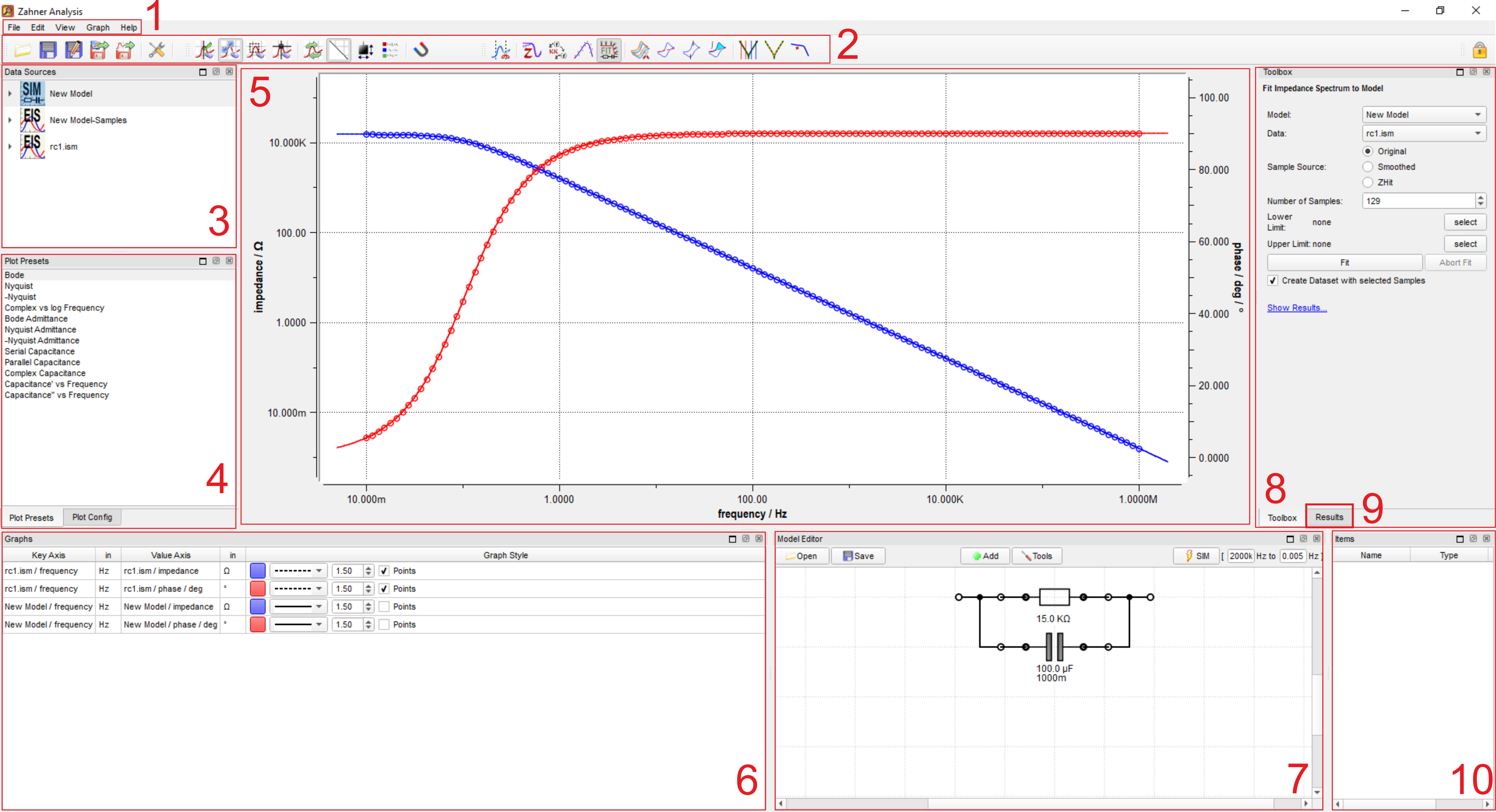
- Menu bar
- Toolbar
- Data Sources window (open files list)
- Plot Presets (plot representations options)
- Main graph area
- Graph (list of open graphs in Graph area)
- Model circuit window –only visible after clicking the “EIS Fit” icon-
- Toolbox
- Results
- Items (cursors and/or label window)
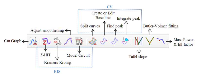
The toolbar consists of many different icons that are designed for use in the evaluation of different electrochemical methods.
In the rest of this section, a step-by-step guide is provided for the evaluation of different electrochemical measurement results. Along with the evaluation, different windows (used during evaluation) are also briefly explained.
4.1 Electrochemical impedance spectroscopy
Electrochemical impedance spectroscopy (EIS) is a widely used electrochemical process that provides insight into the charge transfer steps. To get reliable results from EIS, it is very crucial to fit the impedance spectrum with an equivalent electrical circuit (EEC), which closely mimics the system under investigation. With the Zahner Analysis software, the users can fit the impedance spectrum with an EEC. The software also provides information about the total error in the fitting and the significance of each electrical element used in fitting. This additional information indicates the credibility of the used EEC.
For fitting an EIS spectrum, multiple steps are followed and are explained in detail below
For fitting an EIS spectrum, first open a spectrum using "File" (in Menu bar) and then click "Open". With this, the spectrum will be visible in the Graph area (window 5). The filename of the opened spectrum will be visible in window 3.
The list of the opened graph(s) is presented in window 6. Here color of the graph, its thickness, and format can be modified.
Choose desired graphical representation
For EIS, different graphical representations are possible. A suitable graphical representation can be chosen from window 4. A list of the representations is provided below.
- Bode (Y-axes: |Z| and Phase, X-axis: Frequency)
- Nyquist (Y-axis: Z ՛՛, X-axis: Z ՛)
- -Nyquist (Y-axis: - Z ՛՛, X-axis: Z ՛)
- Complex vs Log Frequency (Y-axes: Z ՛՛ and Z ՛, X-axis: Frequency)
- Bode Admittance (Y-axes: |Y| and Phase, X-axis: Frequency), Here, Y=1/Z
- Nyquist Admittance (Y-axis: Y ՛՛, X-axis: Y ՛)
- -Nyquist Admittance (Y-axis: Y ՛՛, X-axis: - Y ՛)
- Serial Capacitance (Y-axes: Resistance and Serial Capacitance, X-axis: Frequency)
- Parallel Capacitance (Y-axes: Resistance and Parallel Capacitance, X-axis: Frequency)
- Complex Capacitance (Y-axis: C ՛՛, X-axis: C ՛)
- Capacitance vs Frequency (Y-axis: C ՛, X-axis: Frequency)
- Capacitance vs Frequency (Y-axis: C ՛՛, X-axis: Frequency)
Here,
|Z| = Impedance modulus
Z ՛ = Real impedance
Z ՛՛ = Imaginary impedance
Y ՛ = Real admittance
Y ՛՛ = Imaginary admittance
C ՛ = Real capacitance
C ՛՛ = Imaginary capacitance
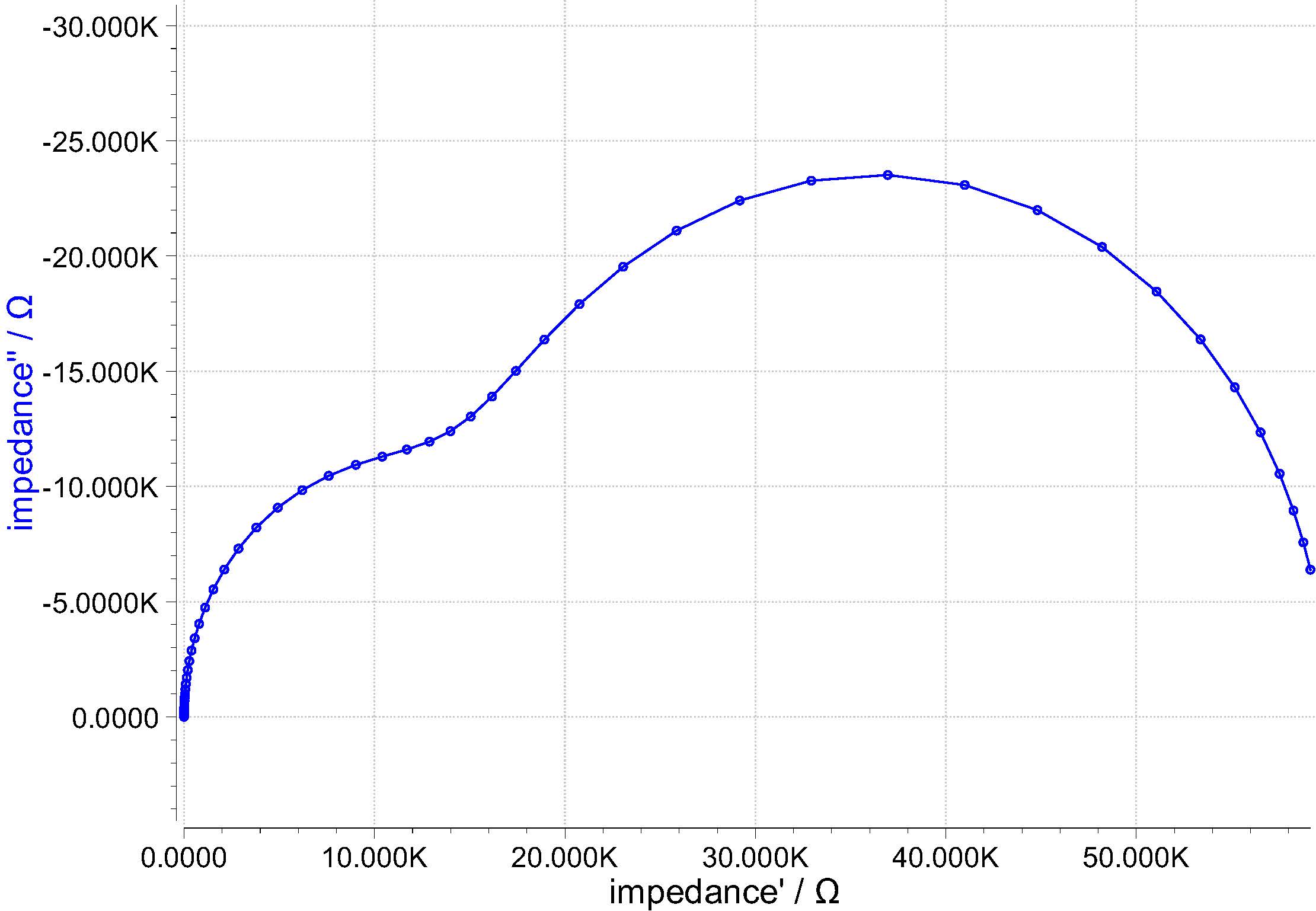
EIS spectrum (Nyquist plot)
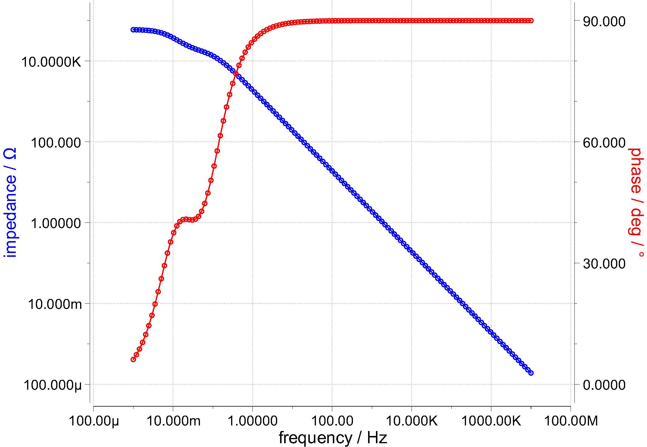
Bode plot
Besides standard Nyquist or Bode-plot representation for the impedance and admittance, there are also additional special graphical representations which are explained below.
Serial Capacitance: In serial capacitance, each impedance point is considered as the sum impedance of a resistor and a capacitor in series. Here,
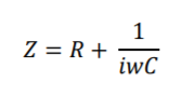
From the formula, the values of the resistance and serial capacitance are calculated.
Parallel Capacitance: In parallel capacitance, each impedance point is considered as the sum impedance of a resistor and a capacitor in parallel. Here,
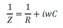
From the formula, the values of the resistance and parallel capacitance are calculated.
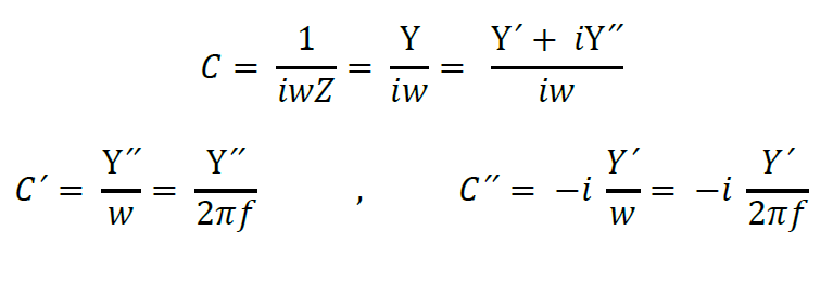
Complex Capacitance: In complex capacitance, real capacitance (C՛) and imaginary capacitances (C՛՛) are defined as follows.
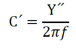
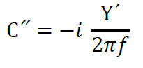
Here Y՛ and Y՛՛ are real and imaginary admittances.
C՛ and C՛՛ are defined as follows.
Real and imaginary capacitances are frequency dependant capacitances and are used for characterizing the supercapacitors. Further information about the real and imaginary capacitances is provided in a research publication titled "Electrochemical Characteristics and Impedance Spectroscopy Studies of Carbon-Carbon Supercapacitors", J. Electrochem. Soc., 150 (3) A292-A300 (2003).
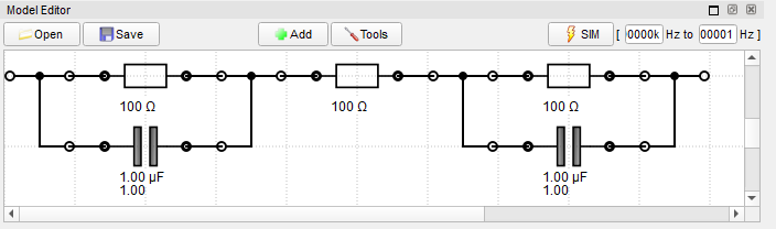
When the desired graphical representation is chosen, then click on the “Model Circuit” icon ( ) in the toolbar. This will open a new window where an EEC can be built.
For generating different electrical elements, click on “Add” and then choose the desired elements. Electrical elements can be connected by connecting the dots. For complex electrical circuits, sometimes the model may look very messy. In such cases, click on “Tools" and then on "Auto Align” to properly align the electrical elements in the model. Once a model circuit is created and the desired frequency range for simulation is provided, then click on  to generate the simulation file (New Model).
After simulating, a “New Model” file is generated in the Data sources window (window 3). To open the file in the Graph window, either double-click on the file or “drag and drop” the file to the Graph window.
Note: In some graphical representation (i.e., the Nyquist plot), you may not be able to see your simulated graph, after opening it in the Graph window. This might be due to the small values assigned to the elements in the equivalent electrical circuit.
For fitting the simulated spectrum to the measured EIS spectrum, click on the Toolbox (window 8). Here different fitting options i) Original, ii) Smoothed, and iii) Z-HIT are available. Choose the desired fitting option and then click “Fit”. This will lead to the fitting of your simulated spectrum. Providing suitable initial values to the electrical elements used in the electrical circuit will help the fitter in properly fitting the spectrum. After fitting, the modified values of electrical elements will be visible in the “Model Circuit” and are also listed in the Results (window 9). Here Value, Significance, and the Fitting Error of each electrical element are also provided. In addition, the “overall Error” of the simulated fitting is also given.
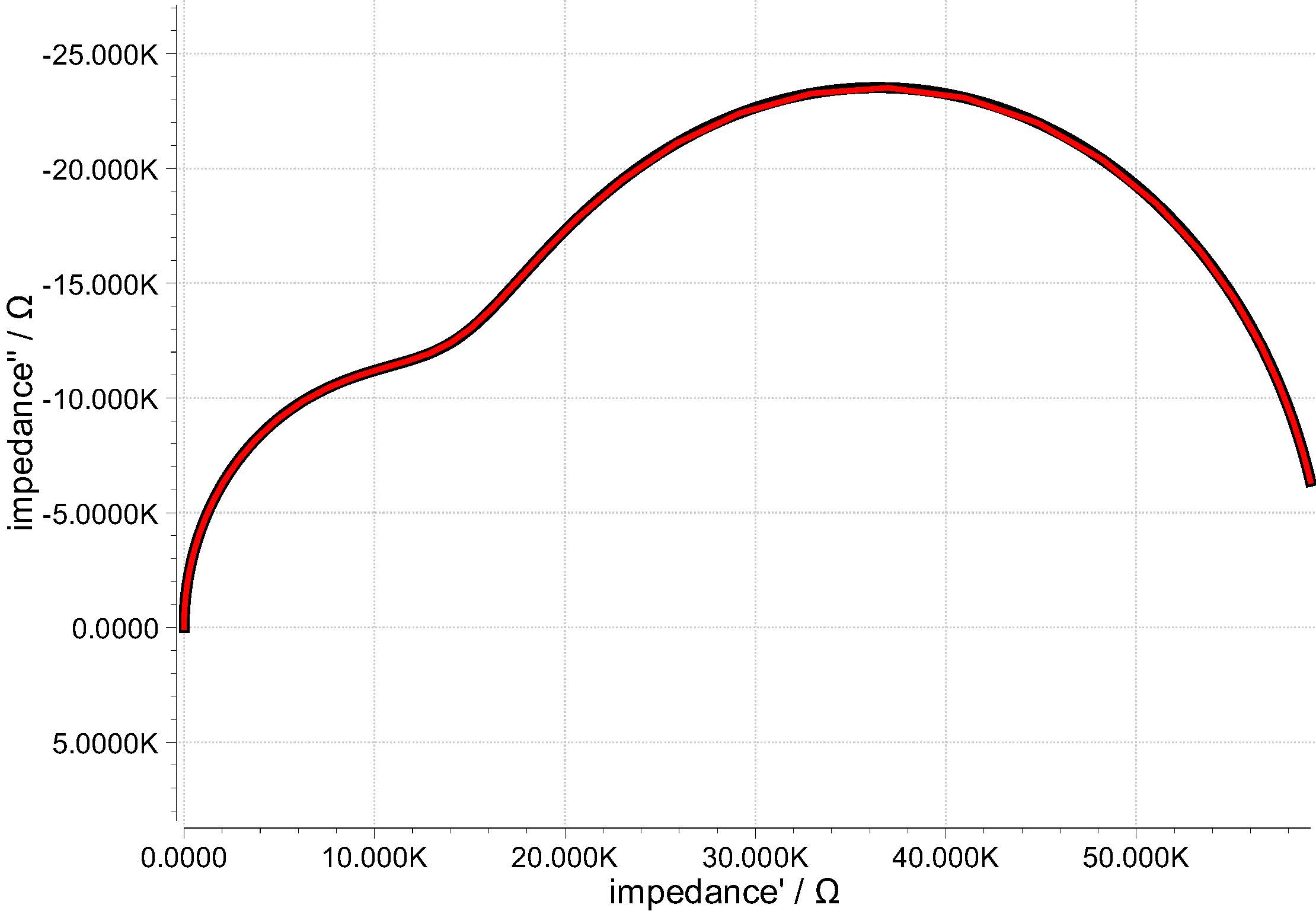
Fitted Nyquist plot
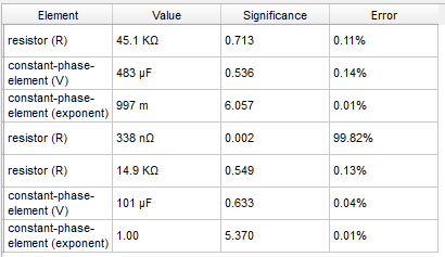
Results window
The simulated spectrum can be saved by clicking "File" in the menu bar and then clicking "Save", or by clicking on the save icon ( ). A text export is also possible.
Note: In the Zahner Analysis software, the data table can also be viewed by right-clicking on the Toolbar and then enabling “Data View”.
4.2 Current-potential (I/E) curve
I/E curves are shown in the Tafel slopes format. Evaluation of the Tafel slope is described in the sections below.
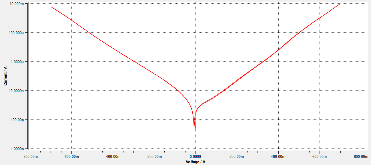
4.2.1 Tafel slope
Tafel slopes are of great importance in electrochemistry and provide insight into the reaction kinetics. In Zahner Analysis software, Tafel slops can be easily calculated from the measured log Current vs potential graph. For measuring the Tafel slope, click on the Tafel slope icon ( ) and then in the Toolbox window, set the 2 cursors for the cathodic arm and 2 cursors for the anodic arm, indicating points between which the slope should be calculated.
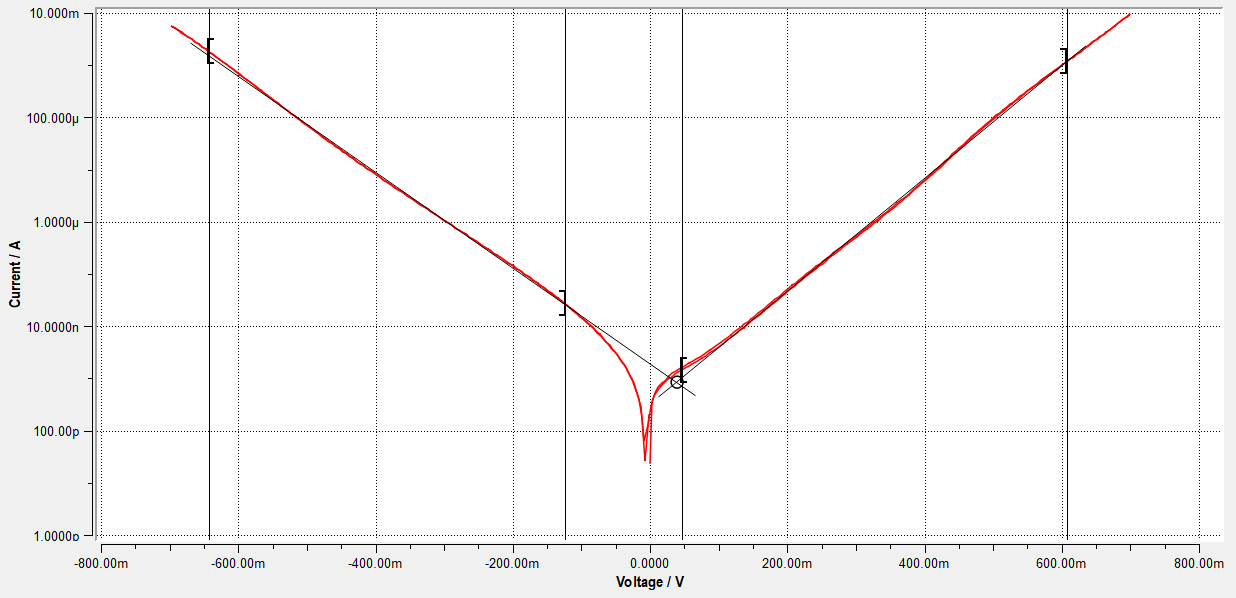
Besides the Tafel slope, the corrosion rate can also be calculated. For the corrosion rate calculation, the user has to provide the Area of Electrode (cm2), Density (g/cm3), and Equivalent Weight (g/mol). The calculated slope and the corrosion rate are shown in the Toolbox window.
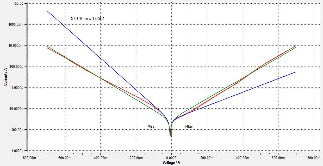
4.2.2 Butler-Volmer
Butler-Volmer (BV) parameters can also be calculated from a log Current vs Potential graph. For calculating the BV parameters, click on the Butler-Volmer icon ( ) and then click on the Toolbox window to set the two cursors on the cathodic and anodic arm to simulate a Butler-Volmer curve. In the image (on right), two simulated BVs are shown. The blue BV is simulated with the two cursors close to the center of the graph, whereas the green BV curve is simulated with the cursors at the far end of the measured BV curve. The results of the simulated curves will be shown in the Toolbox window.
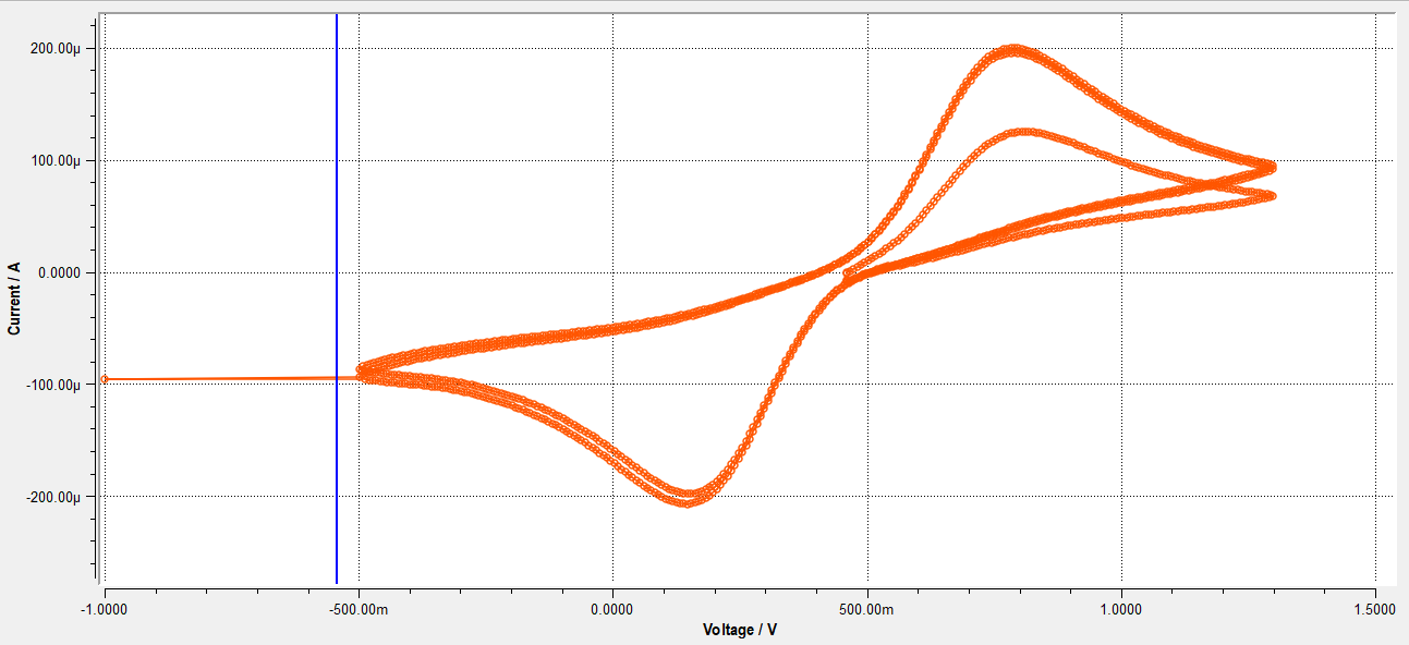
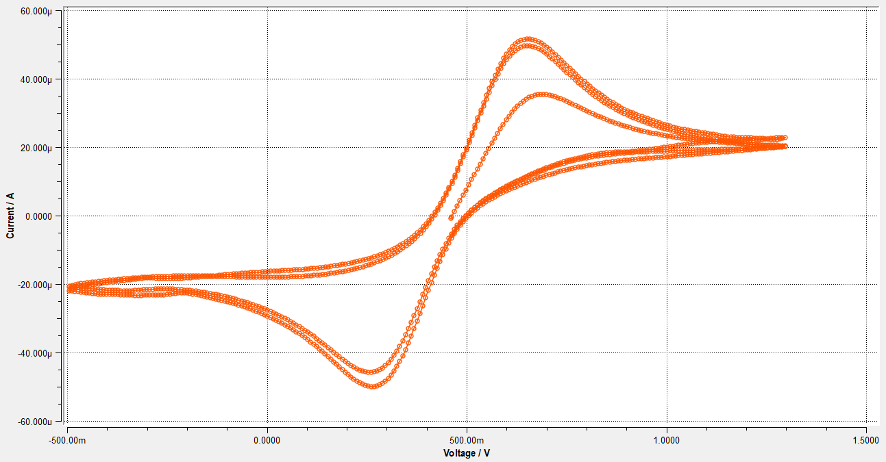
4.3 Cyclic voltammogram
In this subsection, a step by step guide is provided to analyze a cyclic voltammogram (CV) in the Zahner Analysis software.
1. Open the measured CV
Open the measured cyclic voltammogram from the Menu bar by clicking on "File" and then "Open". Like EIS, different representations of the current potential curve are possible and can be set from the "Plot Presets" window (window 4). A list of the available graphic representation is provided below
- Linear I vs U
- Linear I (Linear U) vs time
- Log I vs U
- U vs Log I
- Linear I vs time
- U vs Linear I
- Normalized I vs U
- Norm (sqrt) I vs U
2. Trim the CV
For trimming the artefact on the left side of the CV, first click on the “Cut Graph” icon ( ) and then click on the curve where trimming should be done. Upon clicking, choose a cursor on the graph, and then in the “Toolbox”, click on remove left/right to remove the part on the left or right from the cursor, respectively.
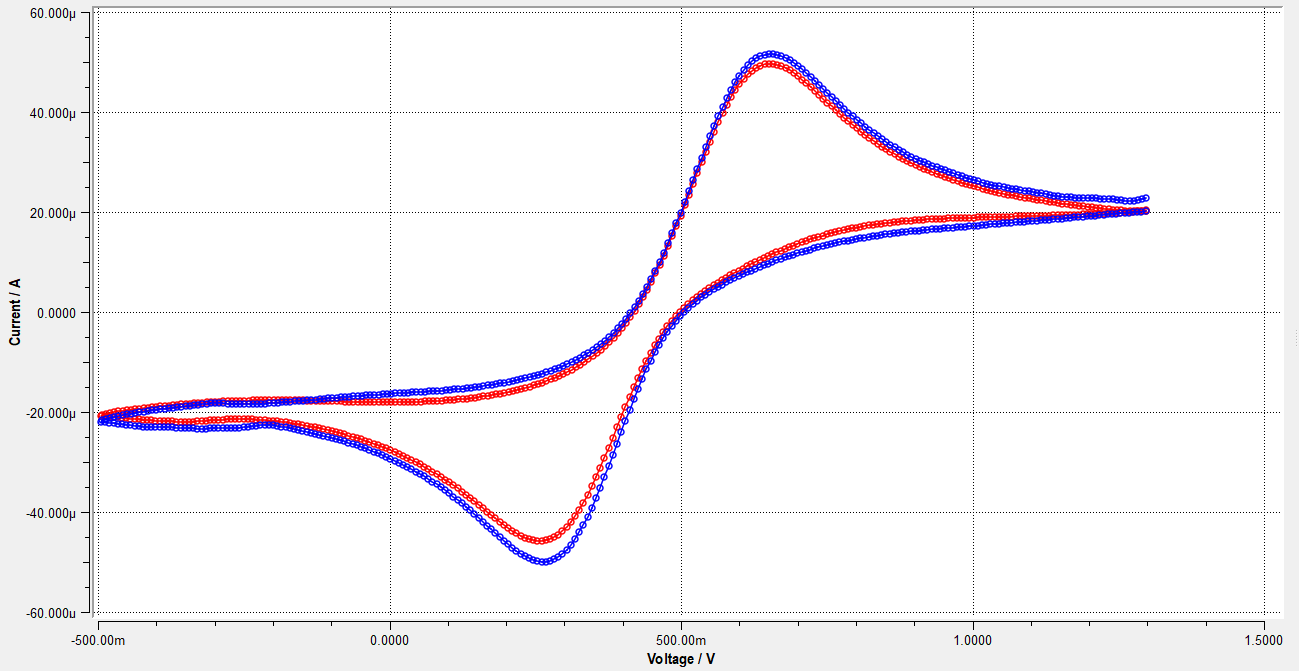
3. Split curve
Split the curve by clicking the icon  and then click “Split” in the Toolbox window. This will split the curve into multiple curves and will assign the splitted curves the pre-decided colors. If the user wants to change the colors then it is possible from the (window 6). Splitting will also generate new files with individual CVs and these files will be listed in the Data Source window (window 3).
For the rest of the evaluation, only one splitted CV will be used.
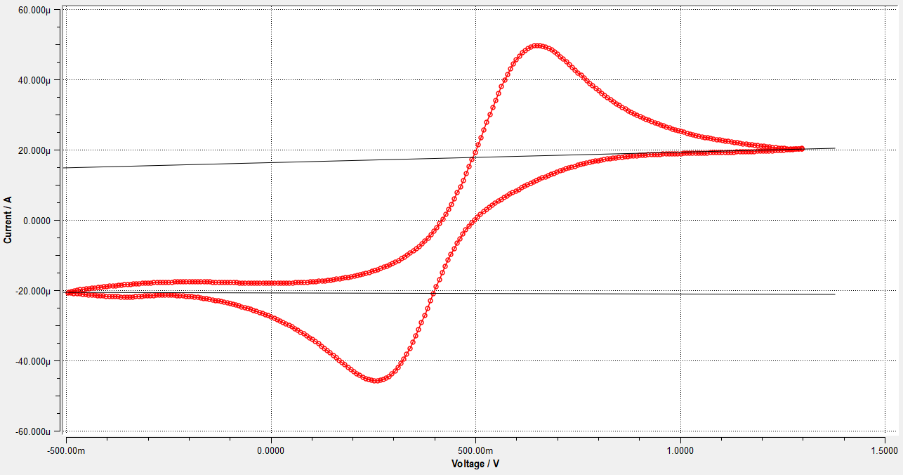
4. Draw the Baseline(s)
Draw the baseline by clicking on the icon ( ) and then sketch the desired baseline on the main graph window. If the user wants to draw more than one baseline then click on “New Baseline” in Toolbox to draw the additional baselines.
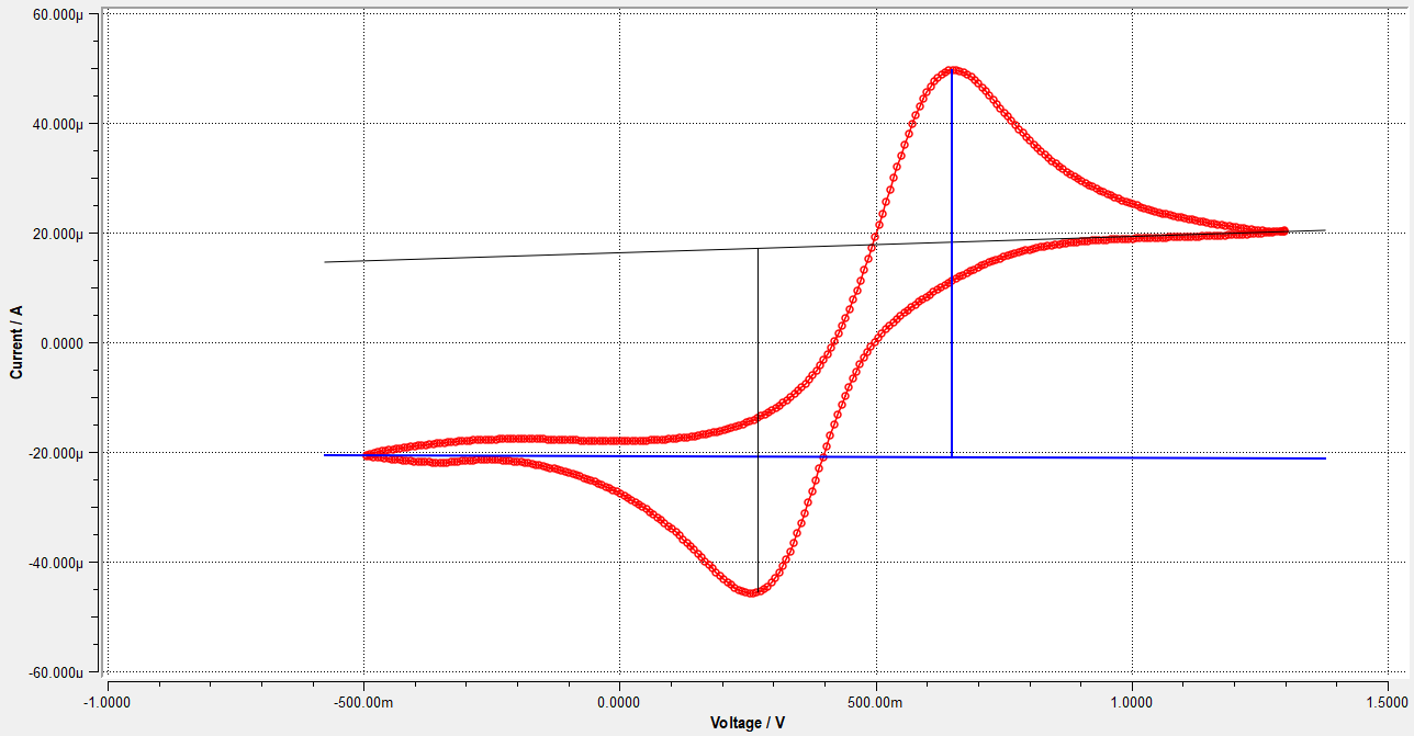
5. Peak position and height
To measure the peak position, click on the peak position icon ( ) and then with the mouse click on the peak of the CV. The peak position and additional information about the peak will be listed in the “Cursor and label" window (window 10).
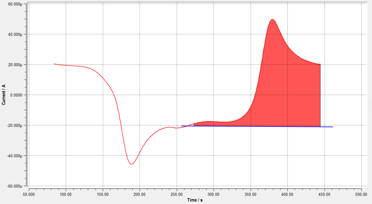
6. Peak area integration
To integrate the area under peak, click on the icon  , then in the “Toolbox” window, set the baseline, “start of peak” and “end of peak”. If previously, a baseline was drawn then that baseline will be automatically chosen. For choosing the start of the peak click the “Select” icon and then on the Graph window click on the CV where the peak is starting and then repeat the same process to select the end of the peak. In the end, clicking on the “Integrate Charge” will integrate the peak. The integrated peak will be shown only “Linear I vs time” representation.
4.3.1 Current-Voltage graph properties
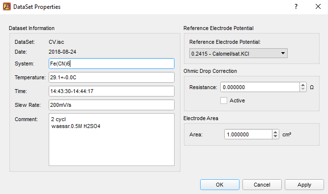
For setting the reference electrode, ohmic drop resistance, and the electrode area, right-click with the mouse on the file name in the “Data Source” window and then click “Properties”. This will open the “Data Set Properties” window where the above-mentioned parameters can be used. In addition, this window also includes comments and technical details which were provided during the measurement in the Thales software.
For reference electrode setting, a user-defined reference electrode option is also provided, where the user can specify the potential of his/her reference electrode which is not available in the list.
To see the changes in the Graph window, by changing the settings in the “Data Set Properties”, window, the graph should be in Current Density (A/cm2) settings and not Current (A) settings. This setting can be changed by clicking on the “Reference Area” icon ( ) in the Toolbar.